From Rolling Quarters to Monthly Estimates: SIDRA Mensalization Guide

Overview

Brazil’s Continuous National Household Sample Survey (PNADC) publishes labor market indicators as rolling (moving) quarters — 3-month moving averages where each published “quarter” shares 2 months with its neighbors. This smoothing hides short-term dynamics: turning points are delayed, seasonal patterns are distorted, and international comparison becomes difficult.

The PNADCperiods package includes a SIDRA mensalization module that recovers exact monthly estimates from rolling quarter data. This vignette explains how to use it.

Why Rolling Quarters Are Problematic

Each published “quarter” is actually a 3-month moving average:

“2019-Q1” = average of Jan, Feb, Mar 2019
“2019-Q2” = average of Feb, Mar, Apr 2019
“2019-Q3” = average of Mar, Apr, May 2019

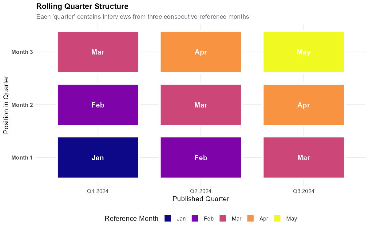
Rolling quarters overlap: each ‘quarter’ shares 2 months with its neighbors

When unemployment jumps sharply in a single month, the rolling quarter spreads that spike across multiple overlapping periods. The mensalization algorithm inverts this averaging process to recover the true monthly values.

Quick Start

library(PNADCperiods)

# Step 1: Fetch rolling quarter data from SIDRA API
rolling_quarters <- fetch_sidra_rolling_quarters()

# Step 2: Convert to monthly estimates
monthly <- mensalize_sidra_series(rolling_quarters)

# Step 3: Use your monthly data!
head(monthly[, .(anomesexato, m_popocup, m_taxadesocup)])

That’s it! You now have monthly estimates starting from January 2012.

fetch_sidra_rolling_quarters() downloaded 86+ economic indicators from IBGE’s SIDRA API
mensalize_sidra_series() applied the mensalization formula using pre-computed starting points (bundled with the package)
The result is a data.table with one row per month and m_* columns for each mensalized series

Understanding the Output

The mensalized output contains:

anomesexato: Month identifier (YYYYMM format, e.g., 201903 = March 2019)
m_* columns: Mensalized (monthly) estimates for each series
Price indices: ipca100dez1993, inpc100dez1993 (passed through for deflation)

Key series include:

Column	Description	Unit
`m_populacao`	Total population	Thousands
`m_pop14mais`	Population 14+ years	Thousands
`m_popocup`	Employed population	Thousands
`m_popdesocup`	Unemployed population	Thousands
`m_taxadesocup`	Unemployment rate	Percent
`m_taxapartic`	Labor force participation rate	Percent
`m_massahabnominaltodos`	Total nominal wage bill	Millions R$

Rate series (like m_taxadesocup) are derived from mensalized level series when compute_derived = TRUE (the default). They are computed as ratios of the mensalized levels, not directly mensalized from the rolling quarter rates.

Discovering Available Series

Use get_sidra_series_metadata() to explore all 86+ available series:

meta <- get_sidra_series_metadata()

# View series organized by theme
meta[, .N, by = .(theme, theme_category)]

# Filter to specific theme categories
meta[theme_category == "employment_type", .(series_name, description)]

The metadata uses a hierarchical taxonomy: theme (top level, e.g., “labor_market”), theme_category (e.g., “employment_type”), and optionally subcategory (e.g., “levels”, “rates”).

Data Flow

The mensalization process follows a three-step pipeline:

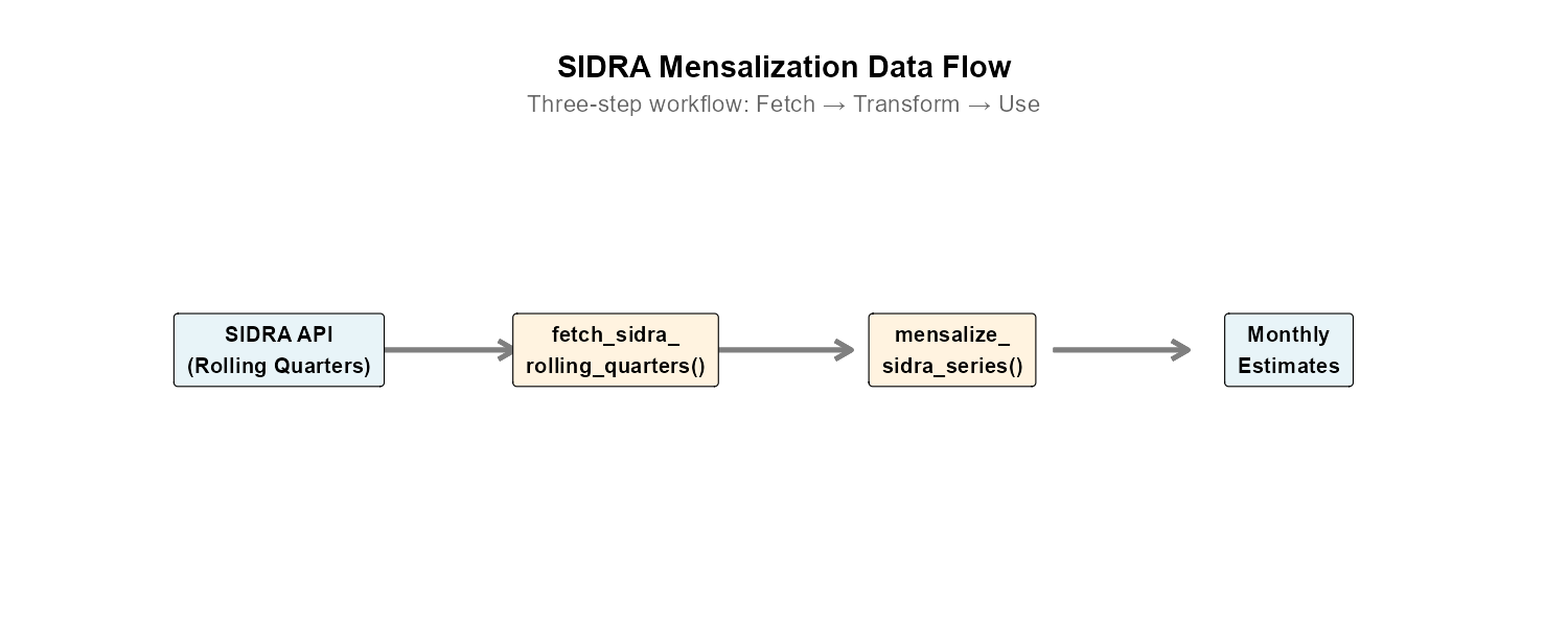
Data flow from SIDRA to monthly estimates

Step 1: Fetching Rolling Quarter Data

fetch_sidra_rolling_quarters() downloads data from five SIDRA tables:

Table	Content
4093	Population and labor force
6390	Income (nominal and real)
6392	Real income by occupation
6399	Employment by sector
6906	Underutilization indicators

rq <- fetch_sidra_rolling_quarters(verbose = TRUE)

# Inspect structure
dim(rq)
names(rq)[1:20]

Key columns: anomesfinaltrimmovel (end month of rolling quarter, YYYYMM), mesnotrim (month position 1/2/3), plus one column per series.

Step 2: The Mensalization Transform

monthly <- mensalize_sidra_series(rq, verbose = TRUE)

# Compare dimensions
cat("Rolling quarters:", nrow(rq), "rows\n")
cat("Monthly data:", nrow(monthly), "rows\n")

The row count is approximately the same (one per month), but the meaning changes from “rolling quarter ending in month X” to “exact estimate for month X”.

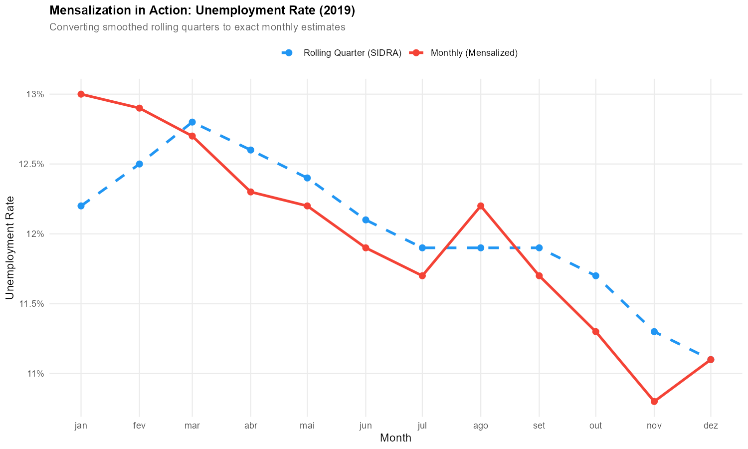
Step 3: Using Monthly Estimates

Show plotting code

# --- VIGNETTE CODE: plot-unemployment ---
library(ggplot2)

monthly[, date := as.Date(paste0(substr(anomesexato, 1, 4), "-",
                                  substr(anomesexato, 5, 6), "-01"))]

ggplot(monthly, aes(x = date, y = m_taxadesocup)) +
  geom_line(color = "#1976D2", linewidth = 0.8) +
  labs(title = "Monthly Unemployment Rate",
       x = NULL, y = "Unemployment Rate (%)")

Population Data for Weighting

For analyses requiring monthly population estimates separately:

pop <- fetch_monthly_population()
head(pop)

Returns a data.table with ref_month_yyyymm and m_populacao columns.

Working with Series

Fetching by Theme

Instead of fetching all 86+ series, filter by theme or theme category:

# Only employment type series
employment <- fetch_sidra_rolling_quarters(theme_category = "employment_type")

# Only wage mass series
wages <- fetch_sidra_rolling_quarters(theme_category = "wage_mass")

# Only labor market theme (includes participation, unemployment, employment types, etc.)
labor <- fetch_sidra_rolling_quarters(theme = "labor_market")

Fetching Specific Series

For maximum efficiency, request only the series you need:

# Only unemployment-related series
unemp <- fetch_sidra_rolling_quarters(
  series = c("popdesocup", "taxadesocup", "popnaforca")
)

Excluding Derived Series

Some series are rates computed from other series. To fetch only “base” series:

# Exclude computed rates (only population and income levels)
base_only <- fetch_sidra_rolling_quarters(exclude_derived = TRUE)

Selecting Output Columns

After mensalization, select columns as needed:

monthly <- mensalize_sidra_series(rq)

# Select specific series
labor_market <- monthly[, .(
  anomesexato,
  employed = m_popocup,
  unemployed = m_popdesocup,
  unemp_rate = m_taxadesocup,
  participation = m_taxapartic
)]

The Mensalization Methodology

This section can be skipped by users who just need results.

The Core Concept

Rolling quarters are 3-month moving averages. If we denote the true monthly value for month $t$ as $y_t$ , then the rolling quarter value $x_t$ is:

$x_t = \frac{y_{t-2} + y_{t-1} + y_t}{3}$

The mensalization algorithm inverts this relationship to recover $y_t$ from the sequence of $x_t$ values.

The Mensalization Formula

Step 1: Compute first differences

$d3_t = x_t - x_{t-1}$

Step 2: Identify month position (mesnotrim)

Each month has a position within its quarter: - Position 1: Jan, Apr, Jul, Oct - Position 2: Feb, May, Aug, Nov - Position 3: Mar, Jun, Sep, Dec

Step 3: Cumulative sum by position

For each position separately, compute the cumulative sum of first differences, starting from a calibrated “starting point” $y_0$ :

$y_t = y_0 + \sum_{s \in \text{same position}, s \leq t} d3_s$

Mensalization process: rolling quarters (blue) vs monthly estimates (red)

The Role of Starting Points ( $y_0$ )

The starting point $y_0$ is crucial. It determines the level of all subsequent monthly estimates. The package includes pre-computed starting points for 53 series, calibrated during the stable 2013-2019 period.

Starting points are computed by:

Processing PNADC microdata to get “true” monthly aggregates ( $z$ values)
Comparing these to rolling quarters
Finding the $y_0$ that makes $y_0 + \text{cumsum}(d3)$ match the microdata

Assumptions and Limitations

Monthly values within each position evolve smoothly
The calibration period (2013-2019) reflects “normal” conditions
Cannot recover intra-month variation
Starting points are calibrated to national totals (not regional breakdowns)

Practical Considerations

API Caching

The package caches SIDRA API responses in memory during your R session:

# First call: fetches from API (~10 seconds)
rq1 <- fetch_sidra_rolling_quarters()

# Second call with use_cache = TRUE: uses cached data (instant)
rq2 <- fetch_sidra_rolling_quarters(use_cache = TRUE)

# Clear all cached data (force fresh fetch on next call)
clear_sidra_cache()

The cache persists until you call clear_sidra_cache() or restart R.

Common Errors

Error	Cause	Solution
“Series not found”	Misspelled series name	Check `get_sidra_series_metadata()`
“API timeout”	SIDRA server slow	Retry; use `use_cache = TRUE`
“No starting points”	Custom series	See Custom Starting Points below

# Check if series exists
meta <- get_sidra_series_metadata()
"taxadesocup" %in% meta$series_name  # TRUE

Data Quality Notes

COVID-19 disruptions (2020): IBGE suspended in-person interviews during the pandemic. Some indicators show unusual patterns in 2020-Q2.

CNPJ series availability: Series based on CNPJ registration (empregadorcomcnpj, contapropriacomcnpj, etc.) are only available from October 2015, when V4019 was introduced.

Custom Starting Points

For users with calibrated PNADC microdata.

Use the bundled starting points (default) unless:

Your series isn’t bundled — Custom variable definitions
Different calibration period — Non-standard reference period
Regional breakdown — State or metro-area mensalization

Option A: All-in-One Function

# Load your stacked PNADC microdata (with pnadc_apply_periods weights)
stacked <- readRDS("my_calibrated_pnadc.rds")

# Compute starting points
custom_y0 <- compute_starting_points_from_microdata(
  data = stacked,
  calibration_start = 201301L,
  calibration_end = 201912L,
  verbose = TRUE
)

# Use custom starting points
monthly <- mensalize_sidra_series(rq, starting_points = custom_y0)

Option B: Step-by-Step

# Step 1: Build crosswalk and calibrate
crosswalk <- pnadc_identify_periods(stacked)
calibrated <- pnadc_apply_periods(
  stacked, crosswalk,
  weight_var = "V1028",
  anchor = "quarter",
  calibration_unit = "month"
)

# Step 2: Compute z_ aggregates (monthly totals from microdata)
z_agg <- compute_z_aggregates(calibrated)

# Step 3: Fetch rolling quarters for comparison
rq <- fetch_sidra_rolling_quarters()

# Step 4: Compute starting points
y0 <- compute_series_starting_points(
  monthly_estimates = z_agg,
  rolling_quarters = rq,
  calibration_start = 201301L,
  calibration_end = 201912L
)

# Step 5: Use custom starting points
result <- mensalize_sidra_series(rq, starting_points = y0)

CNPJ-based series automatically use a later calibration period (2016-2019) when use_series_specific_periods = TRUE (the default in compute_series_starting_points()).

Validating Custom Starting Points

bundled <- pnadc_series_starting_points

# Merge and compare
comp <- merge(custom_y0, bundled,
              by = c("series_name", "mesnotrim"),
              suffixes = c("_custom", "_bundled"))

comp[, rel_diff := abs(y0_custom - y0_bundled) / abs(y0_bundled) * 100]
comp[rel_diff > 1]  # Flag series with >1% difference

Case Study: COVID-19 Unemployment

How quickly did unemployment rise when COVID-19 hit Brazil? Rolling quarter data obscures these dynamics. Monthly estimates reveal the exact timing.

Show analysis code

# --- VIGNETTE CODE: covid-analysis ---
# Fetch all series and mensalize
rq <- fetch_sidra_rolling_quarters()
monthly <- mensalize_sidra_series(rq)

# Filter to COVID period
covid_period <- monthly[anomesexato >= 201901 & anomesexato <= 202212]

# Create date column
covid_period[, date := as.Date(paste0(
  substr(anomesexato, 1, 4), "-",
  substr(anomesexato, 5, 6), "-01"
))]

# Find peak
peak_month <- covid_period[which.max(m_taxadesocup)]
cat("Peak unemployment:", peak_month$m_taxadesocup, "% in",
    format(peak_month$date, "%B %Y"), "\n")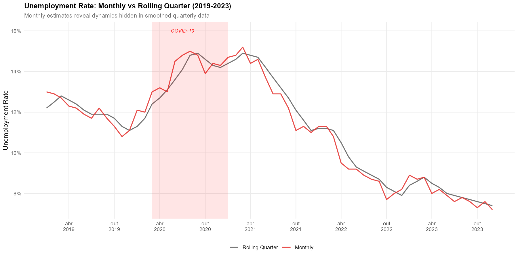

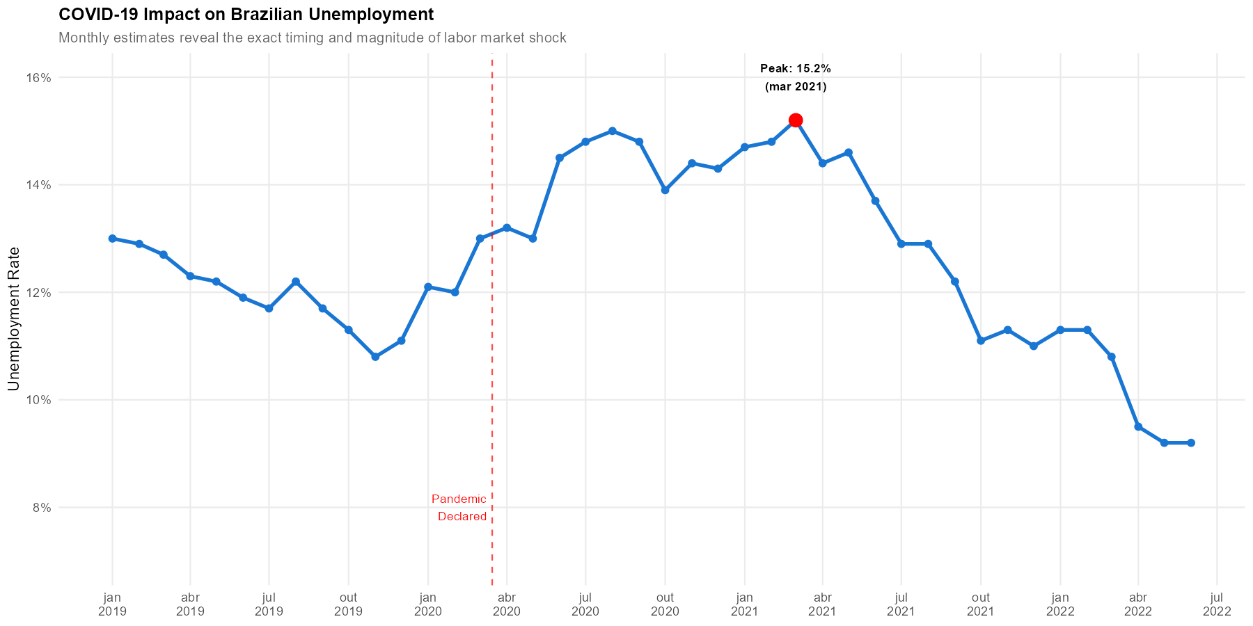
Monthly vs rolling quarter unemployment rate (2019-2023)

COVID-19 impact on Brazilian unemployment

Key findings from monthly estimates:

Exact peak timing: Monthly data pinpoints the peak month, while rolling quarters show only a gradual rise
Speed of impact: The monthly series reveals a sharp spike that rolling quarters smooth over 3+ months
Recovery dynamics: Monthly estimates show pauses and reversals in recovery that are hidden in quarterly averages

Series Naming Conventions

Pattern	Meaning	Example
`m_`	Mensalized monthly estimate	`m_popocup`
`pop*`	Population count	`populacao`, `pop14mais`
`*comcart`	With formal contract	`empregprivcomcart`
`*semcart`	Without formal contract	`empregprivsemcart`
`*comcnpj`	With CNPJ registration	`empregadorcomcnpj`
`taxa*`	Rate (percent)	`taxadesocup`
`nivel*`	Level/ratio (percent)	`nivelocup`
`rend*`	Income (rendimento)	`rendhabnominaltodos`
`massa*`	Wage bill (massa salarial)	`massahabnominaltodos`
`hab`	Usually received (habitual)	`rendhabnominaltodos`
`efet`	Actually received (efetivo)	`rendefetnominaltodos`

For the complete catalog, use get_sidra_series_metadata():

meta <- get_sidra_series_metadata()

# Filter by theme category
meta[theme_category == "employment_type", .(series_name, description)]

# Filter by theme and pattern
meta[theme == "labor_market" & grepl("taxa|nivel", series_name),
     .(series_name, description)]

Function Reference

Function	Purpose
`fetch_sidra_rolling_quarters()`	Download rolling quarter data from SIDRA API
`fetch_monthly_population()`	Get monthly population estimates
`mensalize_sidra_series()`	Convert rolling quarters to monthly estimates
`get_sidra_series_metadata()`	Explore available series and metadata
`clear_sidra_cache()`	Clear cached API data
`compute_z_aggregates()`	Compute monthly aggregates from calibrated microdata
`compute_series_starting_points()`	Compute $y_0$ values from aggregates
`compute_starting_points_from_microdata()`	All-in-one $y_0$ computation

Bundled data: pnadc_series_starting_points — pre-computed $y_0$ for 53 series x 3 month positions (calibration period: 2013-2019).

References

HECKSHER, Marcos. “Valor Impreciso por Mes Exato: Microdados e Indicadores Mensais Baseados na Pnad Continua”. IPEA - Nota Tecnica Disoc, n. 62. Brasilia, DF: IPEA, 2020. https://portalantigo.ipea.gov.br/portal/index.php?option=com_content&view=article&id=35453
HECKSHER, M. “Cinco meses de perdas de empregos e simulacao de um incentivo a contratacoes”. IPEA - Nota Tecnica Disoc, n. 87. Brasilia, DF: IPEA, 2020.
HECKSHER, Marcos. “Mercado de trabalho: A queda da segunda quinzena de marco, aprofundada em abril”. IPEA - Carta de Conjuntura, v. 47, p. 1-6, 2020.
Barbosa, Rogerio J; Hecksher, Marcos. (2026). PNADCperiods: Identify Reference Periods in Brazil’s PNADC Survey Data. R package version v0.1.0. https://github.com/antrologos/PNADCperiods