Monthly Poverty Analysis with Annual PNADC Data

Introduction

When exactly did poverty spike during COVID-19? Official annual statistics tell us that 2020 was a difficult year—but they can’t tell us whether the crisis peaked in April or June, whether the Auxilio Emergencial reduced poverty immediately or with a delay, or what the month-by-month recovery path looked like. Monthly data can.

This vignette combines the mensalization algorithm with annual PNADC data to produce monthly poverty statistics. The annual PNADC releases contain comprehensive household income measures (VD5008) that aren’t available in the quarterly releases. By applying a mensalization crosswalk (built from quarterly data) to annual income data, we get monthly temporal precision with comprehensive income measurement.

Data Workflow: Monthly Poverty Analysis with Annual PNADC

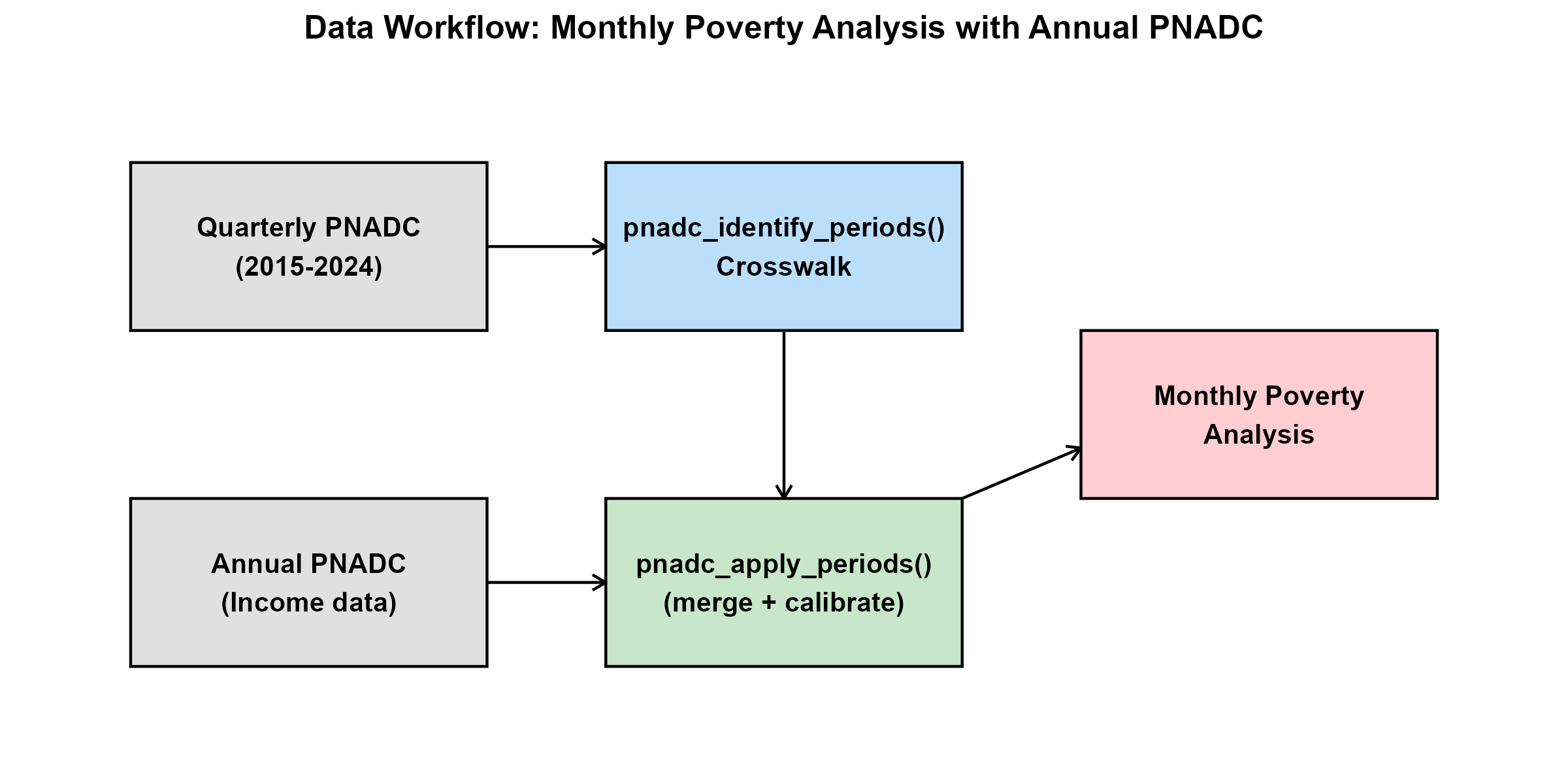
IBGE’s PNADC uses a rotating panel design where the same households appear in both quarterly and annual data. The workflow is:

1. Build a crosswalk from quarterly data using pnadc_identify_periods()
2. Apply the crosswalk to annual income data with pnadc_apply_periods() (which handles the merge internally and calibrates weights)
3. Analyze detailed income and poverty measures at monthly frequency

---

Prerequisites

library(PNADCperiods)
library(data.table)
library(fst)
library(readxl)      # Read IBGE deflator Excel files
library(deflateBR)   # INPC deflator
library(ggplot2)
library(scales)

You also need:

• Quarterly PNADC data (2015-2024) in .fst format for creating the mensalization crosswalk
• Annual PNADC data (2015-2024) in .fst format with income supplement variables
• Deflator file from IBGE documentation (deflator_pnadc_2024.xls)

---

Complete Workflow

Step 1: Create Mensalization Crosswalk

Load stacked quarterly PNADC data and run the mensalization algorithm. See the Download and Prepare Data vignette for details on obtaining and formatting PNADC microdata.

# Define paths
pnad_quarterly_dir <- "path/to/quarterly/data"

# List quarterly files (2015-2024)
quarterly_files <- list.files(
  path = pnad_quarterly_dir,
  pattern = "pnadc_20(1[5-9]|2[0-4])-[1-4]q\\.fst$",
  full.names = TRUE
)

# Variables needed for mensalization
quarterly_vars <- c(
  "Ano", "Trimestre", "UPA", "V1008", "V1014",
  "V2008", "V20081", "V20082", "V2009",
  "V1028", "UF", "posest", "posest_sxi", "Estrato"
)

# Load and stack quarterly data
quarterly_data <- rbindlist(
  lapply(quarterly_files, function(f) {
    read_fst(f, as.data.table = TRUE, columns = quarterly_vars)
  }),
  fill = TRUE
)

# Build the crosswalk (identifies reference periods)
crosswalk <- pnadc_identify_periods(
  quarterly_data,
  verbose = TRUE
)

# Check determination rate (expect ~96% with 40 quarters of data)
crosswalk[, mean(determined_month, na.rm = TRUE)]

Step 2: Load Annual PNADC Data

Annual PNADC files follow a specific naming convention. Note that 2020-2021 use visit 5 (due to COVID-related field disruptions), while other years use visit 1:

pnad_annual_dir <- "path/to/annual/data"

# Define which visit to use for each year
visit_selection <- data.table(
  ano = 2015:2024,
  visita = c(1, 1, 1, 1, 1, 5, 5, 1, 1, 1)  # 2020-2021 use visit 5
)

Why Visit 5 for 2020-2021?

During COVID-19, IBGE suspended in-person data collection. Visit 1 interviews for 2020-2021 have significant quality issues or are unavailable entirely. Visit 5 interviews were conducted later under improved conditions and are the standard choice for COVID-era income and poverty analysis.

# Build file paths
annual_files <- visit_selection[, .(
  file = file.path(pnad_annual_dir, sprintf("pnadc_%d_visita%d.fst", ano, visita))
), by = ano]

# Variables to load
annual_vars <- c(
  # Join keys
  "ano", "trimestre", "upa", "v1008", "v1014",
  # Demographics
  "v2005", "v2007", "v2009", "v2010", "uf", "estrato",
  # Weights and calibration
  "v1032", "posest", "posest_sxi",
  # Household per capita income (IBGE pre-calculated)
  "vd5008"
)

# Load and stack annual data
annual_data <- rbindlist(
  lapply(annual_files[file.exists(file), file], function(f) {
    dt <- read_fst(f, as.data.table = TRUE)
    setnames(dt, tolower(names(dt)))
    cols_present <- intersect(annual_vars, names(dt))
    dt[, ..cols_present]
  }),
  fill = TRUE
)

Step 2b: Standardize Column Names

The annual data has lowercase column names, but pnadc_apply_periods() requires specific casing for the join keys. Standardize before applying the crosswalk:

# pnadc_apply_periods() expects uppercase join keys
key_mappings <- c(
  "ano" = "Ano", "trimestre" = "Trimestre",
  "upa" = "UPA", "v1008" = "V1008", "v1014" = "V1014",
  "v1032" = "V1032", "uf" = "UF", "v2009" = "V2009"
)

for (old_name in names(key_mappings)) {
  if (old_name %in% names(annual_data)) {
    setnames(annual_data, old_name, key_mappings[[old_name]])
  }
}

Note: The calibration columns posest and posest_sxi stay lowercase—the package expects them in that case. Only the join keys (Ano, Trimestre, UPA, V1008, V1014) and weight column (V1032) need uppercase.

Step 3: Apply Crosswalk and Calibrate Weights

Apply the crosswalk to annual data and calibrate weights using pnadc_apply_periods(). The function handles the merge internally using the five join keys (Ano, Trimestre, UPA, V1008, V1014):

d <- pnadc_apply_periods(
  annual_data,
  crosswalk,
  weight_var = "V1032",
  anchor = "year",
  calibrate = TRUE,
  calibration_unit = "month",
  smooth = TRUE,
  verbose = TRUE
)

# Check match rate (expect ~97% with year anchor)
mean(!is.na(d$ref_month_in_quarter))

Why anchor = "year"? Annual PNADC data contains only one visit per household (e.g., visit 1 or visit 5), not all rotation groups like quarterly data. The "year" anchor calibrates the annual weight V1032 to monthly SIDRA population totals while preserving yearly totals.

Step 4: Construct Per Capita Income

Use IBGE’s pre-calculated household per capita income variable:

# Filter to household members only
d <- d[v2005 <= 14 | v2005 == 16]

# Use IBGE's pre-calculated per capita household income
d[, hhinc_pc_nominal := fifelse(is.na(vd5008), 0, vd5008)]

Step 5: Apply Deflation

Convert nominal income to real values using IBGE deflators:

# Load deflator data (from IBGE documentation)
deflator <- readxl::read_excel("path/to/deflator_pnadc_2024.xls")
setDT(deflator)
deflator <- deflator[, .(Ano = ano, Trimestre = trim, UF = uf, CO2, CO2e, CO3)]

# Merge deflators with data
setkeyv(deflator, c("Ano", "Trimestre", "UF"))
setkeyv(d, c("Ano", "Trimestre", "UF"))
d <- deflator[d]

# INPC adjustment factor to reference date (December 2025)
inpc_factor <- deflateBR::inpc(1,
                               nominal_dates = as.Date("2024-07-01"),
                               real_date = "12/2025")

# Apply deflation
d[, hhinc_pc := hhinc_pc_nominal * CO2 * inpc_factor]

Step 6: Define Poverty Line

Calculate the World Bank PPP-based poverty threshold:

# World Bank poverty line: USD 8.30 PPP per day (upper-middle income threshold)
poverty_line_830_ppp_daily <- 8.30

# 2021 PPP conversion factor (World Bank)
# https://data.worldbank.org/indicator/PA.NUS.PRVT.PP?year=2021
usd_to_brl_ppp <- 2.45
days_to_month <- 365/12

# Monthly value in 2021 BRL
poverty_line_830_brl_monthly_2021 <- poverty_line_830_ppp_daily *
                                     usd_to_brl_ppp * days_to_month

# Deflate to December 2025 reference
poverty_line_830_brl_monthly_2025 <- deflateBR::inpc(
  poverty_line_830_brl_monthly_2021,
  nominal_dates = as.Date("2021-07-01"),
  real_date = "12/2025"
)

d[, poverty_line := poverty_line_830_brl_monthly_2025]

Why USD 8.30/day? This is the World Bank’s upper-middle income poverty threshold, appropriate for Brazil. We use the 2021 PPP conversion factor (2.45 BRL per USD) because 2021 is the World Bank’s reference year for the current poverty lines.

---

Analysis Examples

Helper Functions

Before computing poverty measures, we define the FGT family of poverty indices:

# FGT poverty measure family (Foster-Greer-Thorbecke)
# alpha = 0: Headcount ratio (share below line)
# alpha = 1: Poverty gap (average shortfall)
# alpha = 2: Squared poverty gap (sensitive to inequality among poor)
fgt <- function(x, z, w = NULL, alpha = 0) {
  if (is.null(w)) w <- rep(1, length(x))
  if (length(z) == 1) z <- rep(z, length(x))

  idx <- complete.cases(x, z, w)
  x <- x[idx]; z <- z[idx]; w <- w[idx]

  g <- pmax(0, (z - x) / z)
  fgt_val <- ifelse(x < z, g^alpha, 0)

  sum(w * fgt_val) / sum(w)
}

Example 1: Monthly FGT Poverty Measures

Calculate monthly poverty rates using the FGT family:

# Filter to determined observations
d_monthly <- d[!is.na(ref_month_yyyymm)]

# Use calibrated monthly weight (from pnadc_apply_periods())
d_monthly[, peso := weight_monthly]

# Compute monthly poverty statistics
monthly_poverty <- d_monthly[, .(
  # FGT-0 (Headcount ratio)
  poverty_rate = fgt(hhinc_pc, poverty_line, peso, alpha = 0),

  # FGT-1 (Poverty gap)
  poverty_gap = fgt(hhinc_pc, poverty_line, peso, alpha = 1),

  # Mean income
  mean_income = weighted.mean(hhinc_pc, peso, na.rm = TRUE),

  # Sample size
  n_obs = .N

), by = ref_month_yyyymm]

# Add date for plotting
monthly_poverty[, period := as.Date(paste0(
  ref_month_yyyymm %/% 100, "-",
  ref_month_yyyymm %% 100, "-15"
))]

Show plotting code

# Prepare data for plotting
fgt_data <- melt(
  monthly_poverty[, .(period,
                      `PPP 8.30/day` = poverty_rate)],
  id.vars = "period",
  variable.name = "poverty_line",
  value.name = "rate"
)

fgt_gap_data <- melt(
  monthly_poverty[, .(period,
                      `PPP 8.30/day` = poverty_gap)],
  id.vars = "period",
  variable.name = "poverty_line",
  value.name = "gap"
)

# Panel A: Headcount ratio (FGT-0)
p1 <- ggplot(fgt_data, aes(x = period, y = rate, color = poverty_line)) +
  geom_line(linewidth = 0.8) +
  geom_point(size = 1) +
  scale_y_continuous(labels = percent_format(accuracy = 1),
                     limits = c(0, NA)) +
  scale_x_date(date_breaks = "1 year", date_labels = "%Y") +
  scale_color_manual(values = c("PPP 8.30/day" = "#b2182b")) +
  labs(title = "A. Poverty Headcount (FGT-0)",
       subtitle = "Share of population below poverty line",
       x = NULL, y = "Poverty Rate",
       color = "Poverty Line") +
  theme_minimal(base_size = 11) +
  theme(legend.position = "bottom",
        panel.grid.minor = element_blank(),
        plot.title = element_text(face = "bold"))

# Panel B: Poverty gap (FGT-1)
p2 <- ggplot(fgt_gap_data, aes(x = period, y = gap, color = poverty_line)) +
  geom_line(linewidth = 0.8) +
  geom_point(size = 1) +
  scale_y_continuous(labels = percent_format(accuracy = 0.1),
                     limits = c(0, NA)) +
  scale_x_date(date_breaks = "1 year", date_labels = "%Y") +
  scale_color_manual(values = c("PPP 8.30/day" = "#ef8a62")) +
  labs(title = "B. Relative Poverty Gap (FGT-1)",
       subtitle = "Average shortfall as share of poverty line",
       x = NULL, y = "Relative Poverty Gap",
       color = "Poverty Line") +
  theme_minimal(base_size = 11) +
  theme(legend.position = "bottom",
        panel.grid.minor = element_blank(),
        plot.title = element_text(face = "bold"))

# Combine panels
library(patchwork)
fig_fgt <- p1 / p2 +
  plot_annotation(
    title = "Monthly Poverty Measures: Brazil, 2015-2024",
    caption = "Source: PNADC/IBGE. Annual data with monthly reference periods from PNADCperiods.",
    theme = theme(
      plot.title = element_text(face = "bold", size = 14),
      plot.subtitle = element_text(size = 11),
      plot.caption = element_text(size = 9, hjust = 0)
    )
  )
fig_fgt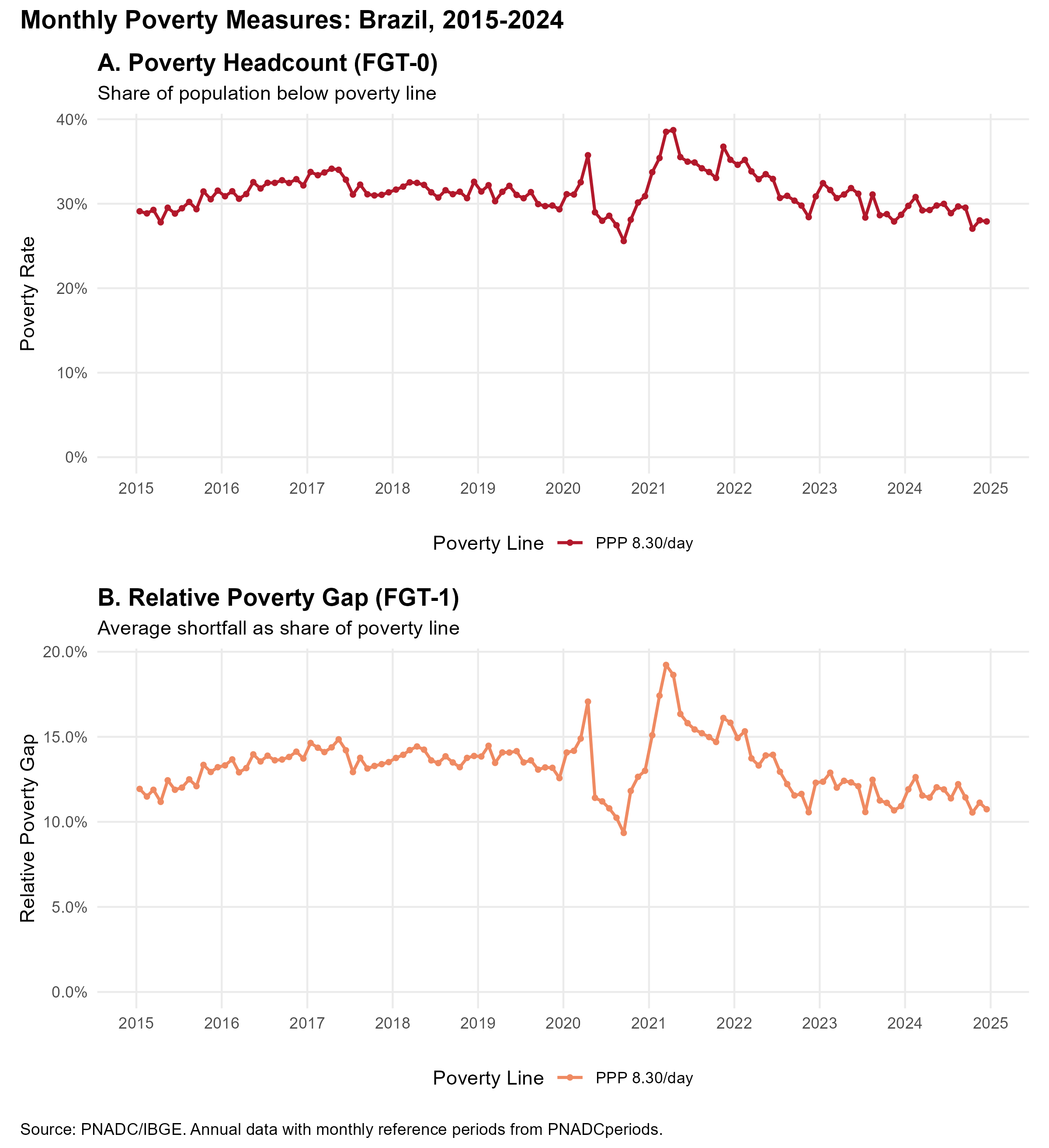

Monthly Poverty Measures: Brazil, 2015-2024

The figure reveals several key dynamics:

1. COVID-19 spike (March-April 2020): The poverty rate shows a sharp increase in early 2020.

2. Auxilio Emergencial effect (May-December 2020): Emergency cash transfers dramatically reduced poverty below pre-pandemic levels.

3. Post-Auxilio adjustment (2021): As emergency aid was reduced, poverty rates partially rebounded.

For proper inference with confidence intervals, use complex survey design with monthly weights—see the Complex Survey Design vignette.

---

Summary

Insight	Annual Data	Monthly Data
COVID poverty spike	Averaged across year	Visible March-April 2020
Auxilio timing	Effect blurred	Clear May 2020 onset
Recovery dynamics	Single 2021 estimate	Monthly trajectory
Seasonal patterns	Invisible	December income spikes

Limitations: ~3% sample loss from undetermined reference months; annual PNADC is released with 18+ month delay; monthly estimates have wider confidence intervals than annual.

---

Further Reading

• Get Started - Basic mensalization workflow
• How It Works - Algorithm details
• Complex Survey Design - Variance estimation
• Applied Examples - Unemployment and minimum wage examples

References

• HECKSHER, Marcos. “Valor Impreciso por Mes Exato: Microdados e Indicadores Mensais Baseados na Pnad Continua”. IPEA - Nota Tecnica Disoc, n. 62. Brasilia, DF: IPEA, 2020. https://portalantigo.ipea.gov.br/portal/index.php?option=com_content&view=article&id=35453
• HECKSHER, M. “Cinco meses de perdas de empregos e simulacao de um incentivo a contratacoes”. IPEA - Nota Tecnica Disoc, n. 87. Brasilia, DF: IPEA, 2020.
• HECKSHER, Marcos. “Mercado de trabalho: A queda da segunda quinzena de marco, aprofundada em abril”. IPEA - Carta de Conjuntura, v. 47, p. 1-6, 2020.
• NERI, Marcelo; HECKSHER, Marcos. “A Montanha-Russa da Pobreza”. FGV Social - Sumario Executivo. Rio de Janeiro: FGV, Junho/2022. https://www.cps.fgv.br/cps/bd/docs/MontanhaRussaDaPobreza_Neri_Hecksher_FGV_Social.pdf
• NERI, Marcelo; HECKSHER, Marcos. “A montanha-russa da pobreza mensal e um programa social alternativo”. Revista NECAT, v. 11, n. 21, 2022.
• IBGE. Pesquisa Nacional por Amostra de Domicilios Continua (PNADC). https://www.ibge.gov.br/estatisticas/sociais/trabalho/
• World Bank. Poverty and Shared Prosperity Reports. Various years.
• Foster, J., Greer, J., & Thorbecke, E. (1984). A class of decomposable poverty measures. Econometrica, 52(3), 761-766.
• Barbosa, Rogerio J; Hecksher, Marcos. (2026). PNADCperiods: Identify Reference Periods in Brazil’s PNADC Survey Data. R package version v0.1.0. https://github.com/antrologos/PNADCperiods