Introduction
This vignette explains how the PNADCperiods algorithm works: the methodology behind converting Brazil’s quarterly PNADC survey into sub-quarterly time series with calibrated weights. For practical usage, see the Get Started vignette.
Policy questions often require sub-quarterly precision that raw PNADC data cannot provide:
- When exactly did unemployment spike during COVID-19? (March 2020 vs. January 2020)
- How quickly did labor markets respond to minimum wage changes? (month-to-month transitions)
- What was poverty in December 2023 specifically? (not just Q4 2023 average)
The algorithm exploits PNADC’s rotating panel design and birthday information to recover this temporal precision. By identifying when each household was actually interviewed within the quarter, we can construct monthly time series with 97% of the original sample retained.
What this vignette covers:
- Why stacked multi-quarter data improves determination from ~70% to ~97%
- The core algorithm: valid interview dates, birthday constraints, UPA-panel aggregation, cross-quarter propagation, dynamic exception detection
- Nested identification hierarchy (months > fortnights > weeks)
- Experimental strategies for improved fortnight/week determination
- Weight calibration and smoothing
- Performance characteristics
Prerequisites: This vignette assumes familiarity with basic PNADC concepts (UPA, rotation groups, survey weights) and focuses on understanding the methodology rather than how to use the functions. For applied examples, see the Applied Examples vignette.
Why Stacked Data Matters
The algorithm achieves 97% determination rate when processing stacked multi-quarter data (full 55-quarter history). If you process quarters individually, you’ll only get ~73% determination.
Why does stacking help? PNADC uses a rotating panel where each household (UPA + V1014) is interviewed for 5 consecutive quarters. Crucially, the same household is always interviewed in the same relative month position (always month 1, always month 2, or always month 3). This means birthday constraints from any quarter can determine the month for all quarters:
UPA=123456, V1014=1 appears in 5 quarters:

  2023-Q1: month_min=1, month_max=2 (ambiguous: Jan or Feb)
  2023-Q2: month_min=1, month_max=3 (ambiguous: Apr, May, or Jun)
  2023-Q3: month_min=2, month_max=2 (DETERMINED: August)  <- Birthday constraint!
  2023-Q4: month_min=1, month_max=2 (ambiguous: Oct or Nov)
  2024-Q1: month_min=2, month_max=3 (ambiguous: Feb or Mar)

Cross-quarter aggregation:
  upa_month_min = max(1, 1, 2, 1, 2) = 2
  upa_month_max = min(2, 3, 2, 2, 3) = 2

Result: ALL 5 quarters -> ref_month_in_quarter = 2
Empirical determination rates by number of quarters stacked (from real PNADC 2012-2025 data):
| Quarters Stacked | Observations | Determination Rate |
|---|---|---|
| 1 (single quarter) | 566,873 | 73.0% |
| 2 | 1,133,889 | 88.2% |
| 4 (1 year) | 2,252,464 | 93.9% |
| 8 (2 years) | 4,530,641 | 96.3% |
| 12 (3 years) | 6,828,144 | 97.1% |
| 20 (5 years) | 11,391,346 | 97.3% |
| 32 (8 years) | 18,088,581 | 97.4% |
| 55 (full history) | 28,395,273 | 97.0% |
The rate peaks around 32 quarters then stabilizes, because the boundary quarters (first 4 and last 4 of any series) have inherently lower rates due to incomplete panel coverage.
Show plotting code (determination rate figure)
p1 <- ggplot(cumulative_det, aes(x = n_quarters, y = det_rate * 100)) +
  geom_line(color = "#2166ac", linewidth = 1.2) +
  geom_point(color = "#2166ac", size = 3.5) +
  geom_hline(yintercept = max(cumulative_det$det_rate) * 100,
             linetype = "dashed", color = "#666666", alpha = 0.7) +
  annotate("text",
           x = max(cumulative_det$n_quarters) * 0.85,
           y = max(cumulative_det$det_rate) * 100 + 1.2,
           label = paste0(sprintf("%.1f%%", max(cumulative_det$det_rate) * 100),
                         " (full history)"),
           color = "#666666", size = 3.5, hjust = 0.5) +
  annotate("text",
           x = 2,
           y = cumulative_det[n_quarters == 1, det_rate * 100] + 2,
           label = paste0(sprintf("%.0f%%", cumulative_det[n_quarters == 1, det_rate * 100]),
                         "\n(single quarter)"),
           color = "#2166ac", size = 3, hjust = 0, vjust = 0) +
  scale_x_continuous(
    breaks = c(1, 10, 20, 30, 40, 50),
    limits = c(0, max(cumulative_det$n_quarters) + 5)
  ) +
  scale_y_continuous(
    breaks = seq(65, 100, by = 5),
    limits = c(60, 100),
    labels = function(x) paste0(x, "%")
  ) +
  labs(
    title = "Monthly Determination Rate Improves with More Quarters Stacked",
    subtitle = paste0("Real PNADC data (2012-", max(quarterly_det$Ano),
                      "): Cross-quarter aggregation exploits rotating panel design"),
    x = "Number of Quarters Stacked",
    y = "Determination Rate"
  ) +
  theme_minimal(base_size = 12) +
  theme(
    plot.title = element_text(face = "bold", size = 14),
    plot.subtitle = element_text(color = "#666666", size = 11),
    panel.grid.minor = element_blank(),
    axis.title = element_text(size = 11),
    plot.margin = margin(10, 20, 10, 10)
  )

p1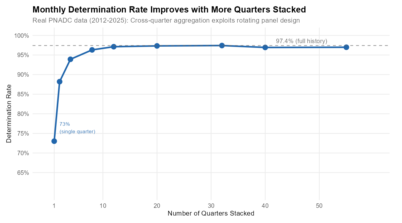
Recommended: Stack at least 2 years (8 quarters) of
data before calling pnadc_identify_periods() to achieve
>96% determination.
The Algorithm Explained
The reference period identification follows a pipeline with shared initial steps and period-specific aggregation:
+-----------------------------------------------------------------------------+
|                    REFERENCE PERIOD IDENTIFICATION PIPELINE                  |
+-----------------------------------------------------------------------------+

INPUTS (per observation):
  Year (Ano), Quarter (Trimestre), Birthday (V2008/V20081/V20082), Age (V2009)
        |
        v
SHARED COMPUTATION (All Periods):
  Step 1: Calculate valid interview Saturdays (IBGE rules)
  Step 2: Apply birthday constraints to narrow date range
  Step 3: Convert dates to period positions (month/fortnight/week)
        |
        v
NESTED IDENTIFICATION (enforced by construction):

  PHASE 1: MONTHS
  |-- Aggregate at (UPA, V1014) level
  |-- CROSS-QUARTER aggregation across ALL quarters
  |-- Dynamic exception detection
  +-- Determination: ~97% (55Q)
                |
                v (only if month determined)
  PHASE 2: FORTNIGHTS
  |-- Aggregate at (Ano, Trimestre, UPA, V1008) level
  |-- NO cross-quarter aggregation
  +-- Determination: ~9% (strict)
                |
                v (only if fortnight determined)
  PHASE 3: WEEKS
  |-- Aggregate at (Ano, Trimestre, UPA, V1008) level
  |-- NO cross-quarter aggregation
  +-- Determination: ~3% (strict)

OUTPUT:
  ref_month_in_quarter (1-3), ref_month_yyyymm (YYYYMM)
  ref_fortnight_in_quarter (1-6), ref_fortnight_yyyyff (YYYYFF)
  ref_week_in_quarter (1-13), ref_week_yyyyww (YYYYWW)
  determined_month, determined_fortnight, determined_week (logical flags)
The identification is nested by construction — fortnights can only be identified if the month is already determined, and weeks only if the fortnight is determined. Months benefit from cross-quarter aggregation, while fortnights and weeks cannot aggregate across quarters. This explains why monthly determination (97%) far exceeds fortnights (9%) and weeks (3%).
Shared Computation (Steps 1-3)
The following three steps are computed once and shared across all period types.
Step 1: Valid Interview Saturdays (IBGE Rules)
IBGE defines that a reference week belongs to a month only if it has at least 4 days within that month. Since reference weeks end on Saturdays, we examine the Saturdays of each month to determine valid interview dates.
How we calculate the first valid Saturday:
first_saturday_day = day of the first Saturday of the month
if first_saturday_day >= 4:
    use this Saturday (it has enough days in the month)
else:
    use the second Saturday (first_saturday_day + 7)
Example for Q1 2023:
JANUARY 2023:
  Sun  Mon  Tue  Wed  Thu  Fri  SAT
   1    2    3    4    5    6   [7]  <- First Saturday is day 7
                                     7 >= 4? YES -> Valid! (7 days in January)

FEBRUARY 2023:
  Wed  Thu  Fri  SAT  ...
   1    2    3   [4]              <- First Saturday is day 4
                                  4 >= 4? YES -> Valid! (4 days in February)

APRIL 2023:
  SAT  Sun  Mon  Tue  ...
  [1]   2    3    4              <- First Saturday is day 1
                                  1 >= 4? NO -> Skip to second Saturday!
  Fri  SAT  Sun  ...
   7   [8]   9                   <- Use day 8 instead
The valid Saturday calculation defines the possible interview
date range for the quarter: - date_min = First
valid Saturday of Month 1 - date_max = First valid Saturday
of Month 3 + 21 days
Step 2: Birthday Constraints
IBGE calculates age using the exact birthdate and the interview reference date. By comparing the calculated age to the birth year, we can determine whether the interview occurred before or after the person’s birthday that year, narrowing the possible interview date window.
visit_before_birthday = (Survey_Year - Birth_Year) - Calculated_Age

If = 0: Interview was AFTER birthday (person already celebrated this year)
If = 1: Interview was BEFORE birthday (birthday hasn't happened yet)
Example: Interview AFTER birthday
Person: Born March 15, 1990
Survey Year and quarter: 2023 Q1
Calculated Age: 33

Check age: 2023 - 1990 = 33
           33 - 33 = 0  -> Interview was AFTER March 15, 2023

New constraint:
  date_min = max(date_min, first_Saturday_on_or_after(March 15))
  date_min = max(Jan 7, March 18) = March 18

This person can only have been interviewed in MARCH (Month 3 of Q1).
Example: Interview BEFORE birthday
Person: Born February 17, 1990
Survey Year and quarter: 2023 Q1
Calculated Age: 32

Check age: 2023 - 1990 = 33
           33 - 32 = 1  -> Interview was BEFORE February 17, 2023

Constraint: date_max = min(date_max, Saturday_before(birthday))
            date_max = min(March 25, February 11) = February 11

This person can only have been interviewed in JANUARY or early FEBRUARY.
Unknown birthdays: When V2008=99, V20081=99, or V20082=9999, that person’s birthday cannot constrain the date. However, they may still be determined through UPA-Panel aggregation (Step 4) or cross-quarter aggregation (Step 5).
Step 3: Date to Period Position
Transform the date window [date_min, date_max] into period positions:
Month positions (1, 2, or 3):
For date_min: if day <= 3 AND not in first month of quarter:
              subtract 1 from month position

For date_max: if day <= 3:
              use the month of (date - 3 days) instead
Boundary handling: Interviews on days 1-3 of a month typically belong to a reference week that started in the previous month.
Fortnight positions (1-6):
fortnight_pos = (month_pos - 1) * 2 + half_of_month
where half_of_month = 1 if day <= 15, else 2| Month | Days 1-15 | Days 16-31 |
|---|---|---|
| 1 | Fortnight 1 | Fortnight 2 |
| 2 | Fortnight 3 | Fortnight 4 |
| 3 | Fortnight 5 | Fortnight 6 |
Week positions (IBGE calendar):
Weeks follow the IBGE calendar convention where weeks run Sunday to Saturday. The first week of a month must have at least 4 days in that month. Reference months contain either 4 or 5 complete weeks.
Month Identification Pipeline (Steps 4-7)
The month identification pipeline uses cross-quarter aggregation to achieve ~97% determination.
Step 4: UPA-Panel Aggregation
All people in the same UPA + V1014 are interviewed together in the same reference month. Take the intersection:
upa_month_min = MAX of all individual month_min_pos
upa_month_max = MIN of all individual month_max_pos
Example:
UPA=123456, Panel V1014=1 has 3 members:

Person A: month_min=1, month_max=2 (could be Jan or Feb)
Person B: month_min=1, month_max=3 (could be Jan, Feb, or Mar)
Person C: month_min=2, month_max=3 (could be Feb or Mar)

Aggregation:
  upa_month_min = max(1, 1, 2) = 2
  upa_month_max = min(2, 3, 3) = 2

Result: min=2, max=2 -> Reference month is FEBRUARY!

Visual:
              Jan    Feb    Mar
Person A:     [=========]
Person B:     [============]
Person C:            [========]
Intersection:        [==]      <- Only February satisfies all
Step 5: Cross-Quarter Aggregation
Since the relative month position is constant across quarters, constraints from any quarter apply to all quarters:
For each (UPA, V1014) group across ALL quarters:
  upa_month_min = MAX of all month_min_pos from all quarters
  upa_month_max = MIN of all month_max_pos from all quarters
This is why processing stacked data improves determination from ~70% (single quarter) to 97% (full history). This cross-quarter aggregation cannot be applied to fortnights or weeks — even though a household is always in the same relative month, the specific fortnight or week within that month varies by quarter.
Step 6: Dynamic Exception Detection
In some quarters, the standard rule (first reference week with at
least 4 days) may produce impossible results
(upa_month_min > upa_month_max). The algorithm detects
these and applies an alternative rule (at least 3 days
instead of 4):
For each UPA-V1014:
  1. Calculate positions using STANDARD rules (>= 4 days)
  2. Also calculate using ALTERNATIVE rules (>= 3 days)
  3. If standard is impossible but alternative works:
     -> Flag which month needs the exception
  4. Propagate: if ANY UPA in the quarter needs exception for a month,
     apply to ALL observations in that quarter
Exception quarters are detected automatically. Examples found in 2012-2025 data: 2016q3, 2016q4, 2017q2, 2022q3, 2023q2, 2024q1.
Step 7: Final Assignment
After applying exceptions: if
upa_month_min == upa_month_max, the reference month is
determined. Otherwise, it remains NA.
What makes observations indeterminate (~3%)?
- Incomplete panel coverage: Boundary quarters (first/last 4 of any series) have UPAs with fewer than 5 visits
- Unit non-response: Fewer responding households means fewer birthday constraints
- Small household sizes or missing birth dates: Fewer constraints to narrow down the month
Indeterminate observations get weight_monthly = NA in
the output (with keep_all = TRUE).
Fortnight and Week Identification
Fortnights and weeks use the same shared computation (Steps 1-3) as months, but with critical differences:
1. They cannot aggregate across quarters. A household’s relative month position is constant (always month 2), but the specific fortnight or week varies by quarter. Therefore constraints are evaluated within each quarter independently.
2. Aggregation key differs. Fortnights and weeks
aggregate at (Ano, Trimestre, UPA, V1008) — household level
within quarter — rather than (UPA, V1014) across
quarters.
3. Nesting is enforced. A fortnight can only be determined if the month is already determined. A week can only be determined if the fortnight is already determined.
Fortnight algorithm:
Fortnights divide the quarter into 6 periods (2 per month). For each
(Ano, Trimestre, UPA, V1008) group, aggregate fortnight
positions. If min == max, the fortnight is determined.
Week algorithm:
Weeks divide the quarter into approximately 13 periods (following the IBGE Sunday-Saturday calendar). Same aggregation logic as fortnights. Determination requires the fortnight to already be known.
| Period | Strict Rate | Aggregation Scope |
|---|---|---|
| Month | 94-97% | Cross-quarter (UPA, V1014) |
| Fortnight | ~9% | Within-quarter (Ano, Trimestre, UPA, V1008) |
| Week | ~3% | Within-quarter (Ano, Trimestre, UPA, V1008) |
Experimental Strategies
For applications requiring larger sub-monthly samples, the package
provides experimental strategies via
pnadc_experimental_periods() that can moderately increase
fortnight and week determination rates.
Important: Experimental strategies produce “likely” assignments based on additional assumptions. They are intended for sensitivity analysis and robustness checks, not for replacing strict determination in rigorous analysis.
| Strategy | Fortnight Rate | Week Rate | Notes |
|---|---|---|---|
| Strict (default) | 8.9% | 3.3% | Definitive determinations only |
| + Probabilistic (conf=0.9) | 13.5% | 3.6% | Conservative probabilistic |
| + Probabilistic (conf=0.8) | 13.5% | 7.5% | Maximum week coverage |
| + UPA Aggregation | 8.9% | 3.3% | No practical improvement |
| + Both (conf=0.9) | 13.5% | 3.6% | Same as probabilistic alone |
Key finding: Probabilistic strategy provides all the improvement. UPA aggregation adds essentially nothing. Choose conf=0.9 for conservative analysis, conf=0.8 for maximum week coverage.
Show plotting code (experimental strategies figure)
# Select key configurations for visualization
exp_plot_data <- experimental_rates[crosswalk_id %in% c(
  "CW-FULL", "EXP-P08", "EXP-P09"
)]

exp_plot_data[, strategy_display := factor(strategy_label,
  levels = c("Strict baseline",
             "Probabilistic (conf=0.8)",
             "Probabilistic (conf=0.9)"),
  labels = c("Strict baseline",
             "Probabilistic (conf=0.8)",
             "Probabilistic (conf=0.9)")
)]

# Reshape to long format
exp_plot_data_long <- melt(exp_plot_data,
  id.vars = "strategy_display",
  measure.vars = c("det_month_overall", "det_fortnight_overall", "det_week_overall"),
  variable.name = "period",
  value.name = "rate"
)

exp_plot_data_long[, period := factor(period,
  levels = c("det_month_overall", "det_fortnight_overall", "det_week_overall"),
  labels = c("Month", "Fortnight", "Week")
)]

exp_plot_data_long[, rate_pct := rate * 100]

# Create bar chart
p_exp <- ggplot(exp_plot_data_long,
                aes(x = period, y = rate_pct, fill = strategy_display)) +
  geom_col(position = "dodge", width = 0.7) +
  geom_text(aes(label = sprintf("%.1f%%", rate_pct)),
            position = position_dodge(width = 0.7),
            vjust = -0.5, size = 3) +
  labs(
    title = "Determination Rates: Strict vs Probabilistic Strategies",
    subtitle = "8-quarter benchmark (2019-2020), 3.76M observations",
    x = NULL,
    y = "Determination Rate (%)",
    fill = "Strategy"
  ) +
  scale_y_continuous(
    limits = c(0, 105),
    breaks = seq(0, 100, by = 20),
    labels = function(x) paste0(x, "%")
  ) +
  scale_fill_manual(values = c(
    "Strict baseline" = "#D55E00",
    "Probabilistic (conf=0.8)" = "#0072B2",
    "Probabilistic (conf=0.9)" = "#009E73"
  )) +
  theme_minimal(base_size = 12) +
  theme(
    plot.title = element_text(face = "bold", size = 14),
    plot.subtitle = element_text(color = "#666666", size = 11),
    legend.position = "bottom",
    panel.grid.major.x = element_blank(),
    panel.grid.minor = element_blank(),
    axis.title = element_text(size = 11),
    plot.margin = margin(10, 20, 10, 10)
  )

p_exp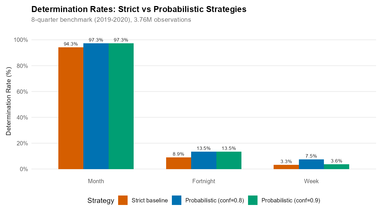
Probabilistic Strategy
When the interview date range spans exactly 2 fortnights or 2 weeks, the probabilistic strategy assigns the period containing the midpoint of the date range.
For each undetermined observation with date range [date_min, date_max]:
  1. Check if range spans exactly 2 periods
  2. Calculate the midpoint: date_midpoint = (date_min + date_max) / 2
  3. Assign the period containing the midpoint
  4. Calculate confidence: based on proportion of range in assigned period
Example:
Person with date range: March 10 - March 20 (within Q1 2023)
Fortnight boundary: March 15/16

Days in fortnight 5 (Mar 1-15):  10, 11, 12, 13, 14, 15 = 6 days
Days in fortnight 6 (Mar 16-31): 16, 17, 18, 19, 20     = 5 days

Date midpoint: March 15 -> Falls in fortnight 5
Confidence: 6/11 ~ 0.55 (55% probability of fortnight 5)
Most probabilistic assignments have relatively low confidence (55-60%), meaning they’re only slightly better than a coin flip. Consider filtering to higher confidence values (>=0.7) for more reliable analysis.
# Build standard crosswalk (store_date_bounds must be TRUE for experimental)
crosswalk <- pnadc_identify_periods(pnadc_stacked, store_date_bounds = TRUE)

# Apply probabilistic strategy with conservative threshold
crosswalk_prob <- pnadc_experimental_periods(
  crosswalk,
  strategy = "probabilistic",
  confidence_threshold = 0.9,
  verbose = TRUE
)

# Check results — experimental assigns determined_probable_* flags
crosswalk_prob[, .(
  strict_fortnight = sum(determined_fortnight),
  probable_fortnight = sum(determined_probable_fortnight, na.rm = TRUE),
  strict_week = sum(determined_week),
  probable_week = sum(determined_probable_week, na.rm = TRUE)
)]

# Filter to strictly determined only (excluding probabilistic)
strict_only <- crosswalk_prob[probabilistic_assignment == FALSE]
UPA Aggregation Strategy
The UPA aggregation strategy exploits a remarkable empirical finding: 100% UPA homogeneity for both fortnights and weeks across 55 quarters of PNADC data (9.6 million household-quarter observations). Whenever a fortnight or week IS strictly determined for any household in a UPA, ALL strictly determined households in that UPA have the SAME period.
Despite this finding, UPA aggregation provides essentially zero improvement in comprehensive testing. Most UPAs already have all households determined (or all undetermined) by the strict algorithm. The strategy cannot create determinations where none exist — it can only propagate existing ones within UPAs.
Recommendation: Use
strategy = "probabilistic" for practical improvements. UPA
aggregation is available for methodological research via
strategy = "upa_aggregation" or
strategy = "both".
Output Columns
pnadc_experimental_periods() adds the following columns
to the crosswalk:
| Column | Type | Description |
|---|---|---|
determined_probable_month |
logical | TRUE if month was assigned by probabilistic strategy |
determined_probable_fortnight |
logical | TRUE if fortnight was assigned by probabilistic strategy |
determined_probable_week |
logical | TRUE if week was assigned by probabilistic strategy |
probabilistic_assignment |
logical | TRUE if any period was assigned experimentally (vs strict) |
Caveats
Low confidence assignments: Mean confidence is ~0.58. Many assignments are only marginally better than random. Consider filtering to confidence >= 0.7.
Neither replaces strict determination: For rigorous causal analysis or official statistics, strict determination should be preferred.
Use
probabilistic_assignmentflag: Filter withcrosswalk[probabilistic_assignment == FALSE]to get strict-only assignments for sensitivity analysis.
Weight Calibration
For sub-quarterly aggregate estimates, you need appropriately
calibrated survey weights. When calibrate = TRUE in
pnadc_apply_periods(), the package:
1. Fetches Monthly Population from SIDRA API
SIDRA (table 6022) provides moving-quarter population estimates (in thousands), not exact monthly values:
| SIDRA Code | 3-Month Window | Represents Population For |
|---|---|---|
| 201203 | Jan+Feb+Mar 2012 | February 2012 |
| 201204 | Feb+Mar+Apr 2012 | March 2012 |
| 201205 | Mar+Apr+May 2012 | April 2012 |
The package shifts values to align with their center month. Boundary months (Jan 2012, latest month) are extrapolated via quadratic regression.
2. Applies Hierarchical Rake Weighting
Calibration cells are nested:
| Cell Level | Definition | Purpose |
|---|---|---|
celula1 |
Age groups: 0-13, 14-29, 30-59, 60+ | Demographic balance |
celula2 |
Post-stratum group + age | Regional-demographic balance |
celula3 |
State (UF) + celula2 | State-level balance |
celula4 |
Post-stratum (posest) + celula2 | Fine geographic balance |
The number of cell levels depends on sample size at each granularity:
| Calibration Unit | Det. Rate | Cell Levels | Smoothing Window |
|---|---|---|---|
| Month | 94-97% | 4 levels (celula1-4) | 3-period rolling mean |
| Fortnight | ~9% | 2 levels (celula1-2) | 7-period rolling mean |
| Week | ~3% | 1 level (celula1 only) | No smoothing |
3. Calibrates to Monthly Population Totals
Final scaling ensures monthly weighted totals match SIDRA population (~206 million average).
Weight Smoothing
The smooth parameter in
pnadc_apply_periods() (default: FALSE) applies
a rolling mean to cell-level calibration adjustments, reducing
artificial quarterly patterns in the weights.
When to enable smoothing
(smooth = TRUE):
- Computing time series for publication or visualization
- Analyzing gradual trends (employment growth, demographic shifts)
When to keep smoothing disabled (default):
- Analyzing rapid shocks (COVID-19 lockdown, sudden policy changes)
- Studying immediate month-to-month changes
- Comparing specific months across years
# Monthly calibration (default)
result <- pnadc_apply_periods(pnadc_stacked, crosswalk,
                               weight_var = "V1028",
                               anchor = "quarter",
                               calibrate = TRUE)

# With smoothing for trend analysis
result_smooth <- pnadc_apply_periods(pnadc_stacked, crosswalk,
                                      weight_var = "V1028",
                                      anchor = "quarter",
                                      smooth = TRUE)

# Fortnight calibration (simplified raking)
result_fn <- pnadc_apply_periods(pnadc_stacked, crosswalk,
                                  weight_var = "V1028",
                                  anchor = "quarter",
                                  calibration_unit = "fortnight")
Handling Indeterminate Observations
By default (keep_all = TRUE), all input rows are
returned. Indeterminate observations get
weight_monthly = NA:
# All rows returned (default keep_all = TRUE)
result <- pnadc_apply_periods(pnadc_stacked, crosswalk,
                               weight_var = "V1028",
                               anchor = "quarter")

# Filter to determined observations for analysis
monthly_pop <- result[!is.na(weight_monthly), .(
  population = sum(weight_monthly, na.rm = TRUE)
), by = ref_month_yyyymm]
Performance
Benchmarks
Period Identification
(pnadc_identify_periods()):
| Dataset Size | Rows | Time | Throughput |
|---|---|---|---|
| 1 quarter | ~570K | ~1.5 sec | ~380K rows/sec |
| 1 year | ~2.3M | ~5 sec | ~460K rows/sec |
| 14 years (2012-2025) | 28.4M | ~2.5 minutes | ~177K rows/sec |
Experimental Strategies
(pnadc_experimental_periods()):
| Strategy | Time | Notes |
|---|---|---|
| probabilistic | ~220 sec | Requires recalculating date bounds |
| upa_aggregation | ~15 sec | Fast aggregation only |
| both | ~235 sec | Sequential application |
Determination Rates by Year
Based on real PNADC data (2012-2025, 55 quarters, 28.4M observations):
| Period | Rate | Notes |
|---|---|---|
| 2013-2019 | 97-99% | Best period (stable data collection) |
| 2020-2021 | 93-96% | COVID-19 degraded IBGE collection |
| 2022-2024 | 95-97% | Post-pandemic normalization |
| Boundary quarters | 70-93% | First/last 4 quarters of any series |
Why boundary quarters have lower rates: In PNADC’s rotating panel (5 visits over 5 quarters), the boundary quarters of any consecutive series include UPA-V1014 groups with fewer than 5 visits in the data. For example, in a dataset of 9 consecutive quarters, only the 5th quarter has full panel utilization — households on their 1st through 5th visit all have complete histories.
Tips and Best Practices
Stack data first: Load 2+ years before calling
pnadc_identify_periods()to maximize determination rate.Validate inputs: Use
validate_pnadc()to catch missing columns early.Check rates by year: Rates should be ~96-99% for 2013-2019. Lower rates suggest data issues or boundary effects.
Handle indeterminate observations: Use
keep_all = TRUE(default) to preserve all observations; indeterminate ones getNAweights.Verify population totals: Monthly weighted sums should approximate Brazil’s population (~206 million in 2024).
Further Reading
- Get Started - Basic workflow for using PNADCperiods
- Applied Examples - COVID, recession, and minimum wage validation
- Annual Poverty Analysis - Monthly poverty with annual PNADC data
- Complex Survey Design - Standard errors and confidence intervals
- IBGE PNADC Documentation
- Package function reference:
?pnadc_identify_periods,?pnadc_apply_periods - Source code: GitHub repository
References
-
HECKSHER, Marcos; BARBOSA, Rogerio J. “Estimation of exact months for the microdata and rolling quarter series from PNAD Continua”. SocArXiv preprint, 2026. https://osf.io/preprints/socarxiv/fra5u_v1
Earlier formulations of the methodology:
- HECKSHER, Marcos. “Valor Impreciso por Mes Exato: Microdados e Indicadores Mensais Baseados na Pnad Continua”. IPEA - Nota Tecnica Disoc, n. 62. Brasilia, DF: IPEA, 2020. https://portalantigo.ipea.gov.br/portal/index.php?option=com_content&view=article&id=35453
- HECKSHER, M. “Cinco meses de perdas de empregos e simulacao de um incentivo a contratacoes”. IPEA - Nota Tecnica Disoc, n. 87. Brasilia, DF: IPEA, 2020.
- HECKSHER, Marcos. “Mercado de trabalho: A queda da segunda quinzena de marco, aprofundada em abril”. IPEA - Carta de Conjuntura, v. 47, p. 1-6, 2020.
Barbosa, Rogerio J; Hecksher, Marcos. (2026). PNADCperiods: Identify Reference Periods in Brazil’s PNADC Survey Data. R package version v0.1.2. https://CRAN.R-project.org/package=PNADCperiods