Overview
The PNADCperiods package converts Brazil’s quarterly
PNADC (Pesquisa Nacional por Amostra de Domicilios Continua) survey data
into sub-quarterly time series. PNADC quarterly statistics are actually
moving averages of three months, which obscures the true timing of
economic shocks, the actual magnitude of changes, and turning points in
trends.
The package offers two complementary approaches:
Microdata mensalization — Identify which specific month, fortnight, or week each survey observation refers to, then calibrate weights for sub-quarterly analysis. Use this for custom variables, subgroup analysis, or individual-level regressions.
SIDRA mensalization — Convert IBGE’s published rolling quarter aggregate series (86+ indicators) into exact monthly estimates. No microdata needed — just 3 lines of code.
For a detailed explanation of the algorithm, see How PNADCperiods Works.
Installation
# From CRAN
install.packages("PNADCperiods")

# Development version from the `dev` branch on GitHub
# remotes::install_github("antrologos/PNADCperiods", ref = "dev")Dependencies: data.table,
checkmate, and sidrar (for weight calibration
and SIDRA API access).
Microdata Mensalization
Use the microdata workflow when you need custom variable definitions, subgroup analysis, individual-level regressions, or indicators not available via SIDRA. This requires PNADC microdata files — see Download and Prepare Data for how to obtain them.
Required Columns
The algorithm needs these columns from your PNADC data:
| Column | Description |
|---|---|
Ano |
Survey year |
Trimestre |
Quarter (1-4) |
UPA |
Primary Sampling Unit |
V1008 |
Household identifier |
V1014 |
Panel identifier (rotation group 1-8) |
V2008 |
Birth day (1-31, or 99 for unknown) |
V20081 |
Birth month (1-12, or 99 for unknown) |
V20082 |
Birth year (or 9999 for unknown) |
V2009 |
Age |
For weight calibration, you also need: V1028 (or
V1032 for annual data), UF,
posest, and posest_sxi.
Step 1: Build the Crosswalk
# Load your stacked quarterly PNADC data
pnadc <- fread("pnadc_stacked.csv")
# Identify reference periods (month, fortnight, week)
crosswalk <- pnadc_identify_periods(pnadc, verbose = TRUE)
Stack multiple quarters for best results. The algorithm exploits PNADC’s rotating panel design — each household (UPA + V1014) is interviewed across 5 consecutive quarters at the same relative month position. Cross-quarter aggregation achieves ~97% month determination from the full 2012-2025 history, vs ~70% from a single quarter.
# Check determination rates
crosswalk[, .(
  month_rate = mean(determined_month),
  fortnight_rate = mean(determined_fortnight),
  week_rate = mean(determined_week)
)]
See ?pnadc_identify_periods for full documentation of
all crosswalk output columns.
Step 2: Apply Crosswalk and Calibrate Weights
result <- pnadc_apply_periods(
  pnadc_2023q1,
  crosswalk,
  weight_var = "V1028",
  anchor = "quarter",
  calibrate = TRUE,
  calibration_unit = "month"
)
Key parameters:
| Parameter | Values | Default |
|---|---|---|
weight_var |
"V1028" (quarterly) or "V1032"
(annual) |
Required |
anchor |
"quarter" or "year"
|
Required |
calibrate |
TRUE / FALSE
|
TRUE |
calibration_unit |
"month", "fortnight",
"week"
|
"month" |
smooth |
TRUE / FALSE
|
FALSE |
Weight calibration adjusts survey weights to match known population
benchmarks from SIDRA, ensuring monthly totals are consistent. The
result includes all original columns plus reference period indicators
and calibrated weights (e.g., weight_monthly).
Step 3: Compute Monthly Estimates
# Monthly unemployment rate
monthly_unemployment <- result[determined_month == TRUE, .(
  unemployment_rate = sum((VD4002 == 2) * weight_monthly, na.rm = TRUE) /
                      sum((VD4001 == 1) * weight_monthly, na.rm = TRUE)
), by = ref_month_yyyymm]

# Monthly population
monthly_pop <- result[, .(
  population = sum(weight_monthly, na.rm = TRUE)
), by = ref_month_yyyymm]
Use determined_month == TRUE (or equivalently,
!is.na(weight_monthly)) to filter to observations with
determined reference months.
For complete analysis examples with plots, see Applied Examples.
Build Once, Apply Many
The crosswalk only needs identification columns, so you can build it once and reuse it:
# Build crosswalk once from stacked data
crosswalk <- pnadc_identify_periods(pnadc_stacked)
saveRDS(crosswalk, "crosswalk.rds")

# Apply to any quarterly or annual dataset
crosswalk <- readRDS("crosswalk.rds")
result_q1 <- pnadc_apply_periods(pnadc_2023q1, crosswalk,
                                  weight_var = "V1028", anchor = "quarter")
result_annual <- pnadc_apply_periods(pnadc_annual_2023, crosswalk,
                                      weight_var = "V1032", anchor = "year")
Monthly Series from SIDRA — No Microdata Needed
If you need aggregate monthly labor market statistics (unemployment rate, employment levels, income), you can get them directly from IBGE’s published data without any microdata. The SIDRA module converts the rolling quarter series published by IBGE into exact monthly estimates.
Quick Start
# Step 1: Fetch rolling quarter data from SIDRA API
rolling_quarters <- fetch_sidra_rolling_quarters()

# Step 2: Convert to exact monthly estimates
monthly <- mensalize_sidra_series(rolling_quarters)

# Step 3: Use your monthly data
head(monthly[, .(anomesexato, m_popocup, m_taxadesocup)])
fetch_sidra_rolling_quarters() downloads 70+ economic
indicators from IBGE’s SIDRA API (Tables 4093, 6390, 6392, 6399, 6906).
mensalize_sidra_series() applies the mensalization formula
using pre-computed starting points bundled with the package, converting
rolling quarter averages into exact monthly values.
The output contains anomesexato (month in YYYYMM format)
and m_* columns with mensalized monthly estimates, starting
from March 2012.
Discovering Available Series
# Browse all 86+ available series
meta <- get_sidra_series_metadata()
meta[, .(series_name, description, unit)]
Most commonly used series:
| Column | Description | Unit |
|---|---|---|
m_taxadesocup |
Unemployment rate | Percent |
m_popocup |
Employed population | Thousands |
m_taxapartic |
Labor force participation rate | Percent |
m_massahabnominaltodos |
Total nominal wage bill | Millions R$ |
m_rendhabnominaltodos |
Average nominal usual income | R$ |
m_taxacompsubutlz |
Composite underutilization rate | Percent |
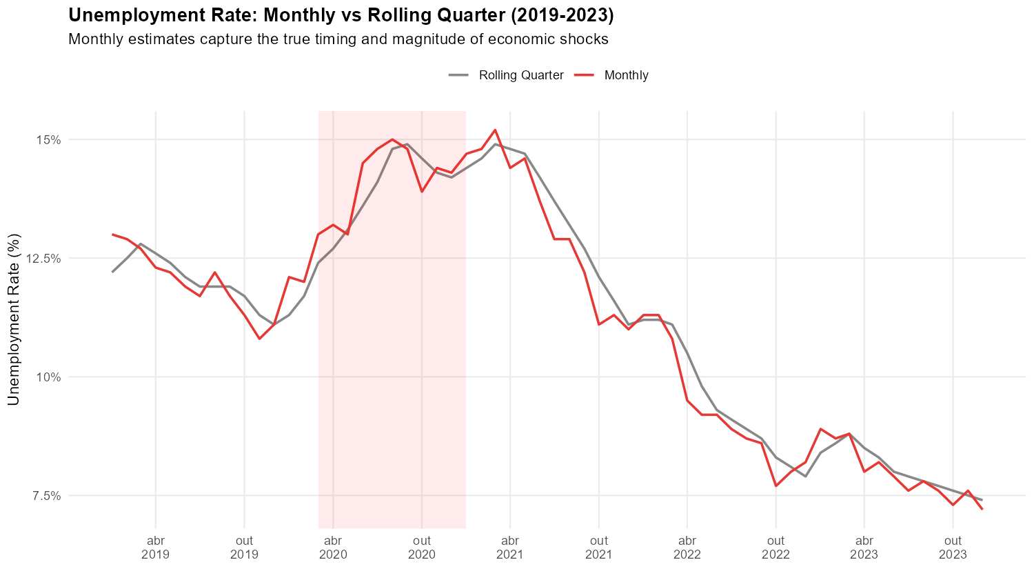
Visualizing Monthly vs Rolling Quarter Data
Since we have both the original rolling quarter data and the mensalized monthly estimates, comparing them is straightforward:
Show plotting code
library(ggplot2)

# Prepare comparison data (merge rolling quarter and monthly estimates)
plot_data <- merge(
  rolling_quarters[, .(anomesexato = anomesfinaltrimmovel, rolling = taxadesocup)],
  monthly[, .(anomesexato, monthly = m_taxadesocup)],
  by = "anomesexato"
)[anomesexato >= 201901 & anomesexato <= 202312]

plot_data[, date := as.Date(paste0(substr(anomesexato, 1, 4), "-",
                                    substr(anomesexato, 5, 6), "-01"))]

# Reshape to long format
plot_long <- melt(plot_data, id.vars = c("anomesexato", "date"),
                  variable.name = "type", value.name = "rate")
plot_long[, type := factor(type,
                           levels = c("rolling", "monthly"),
                           labels = c("Rolling Quarter", "Monthly"))]

# Plot
ggplot(plot_long, aes(x = date, y = rate, color = type)) +
  geom_line(linewidth = 0.8) +
  annotate("rect", xmin = as.Date("2020-03-01"), xmax = as.Date("2020-12-31"),
           ymin = -Inf, ymax = Inf, fill = "red", alpha = 0.08) +
  scale_color_manual(values = c("Rolling Quarter" = "#888888",
                                "Monthly" = "#E53935"),
                     name = NULL) +
  scale_x_date(date_breaks = "6 months", date_labels = "%b\n%Y") +
  scale_y_continuous(labels = function(x) paste0(x, "%")) +
  labs(
    title = "Unemployment Rate: Monthly vs Rolling Quarter (2019-2023)",
    subtitle = "Monthly estimates capture the true timing and magnitude of economic shocks",
    x = NULL,
    y = "Unemployment Rate (%)"
  ) +
  theme_minimal(base_size = 11) +
  theme(
    plot.title = element_text(face = "bold"),
    legend.position = "top",
    panel.grid.minor = element_blank()
  )
For the full SIDRA guide — including custom starting points, methodology, and a COVID case study — see the SIDRA Mensalization Guide.
Improving Determination Rates
PNADC uses a rotating panel where each household (UPA + V1014) is interviewed in 5 consecutive quarters, always at the same relative month position. This means birthday constraints from any quarter can determine the month for all quarters — which is why stacking more data dramatically improves rates:
| Data Stacked | Month Rate | Fortnight Rate | Week Rate |
|---|---|---|---|
| 1 quarter | ~70% | ~7% | ~2% |
| 8 quarters (2 years) | ~94% | ~9% | ~3% |
| 55 quarters (full 2012-2025) | 97.0% | 9.2% | 3.3% |
Fortnight and week rates remain low regardless of stacking because their constraints cannot aggregate across quarters — only month benefits from the panel design.
For analyses requiring higher determination, experimental strategies make informed probabilistic assignments:
# Build crosswalk with date bounds for experimental strategies
crosswalk <- pnadc_identify_periods(pnadc, store_date_bounds = TRUE)

# Apply experimental strategies
crosswalk_exp <- pnadc_experimental_periods(
  crosswalk,
  strategy = "both",
  confidence_threshold = 0.9
)
With strategy = "both" and
confidence_threshold = 0.9, month determination improves to
~97.3% and fortnight to ~13.5%. See How
PNADCperiods Works for details on experimental strategies.
Annual Data
Annual PNADC data uses different weights and achieves higher determination rates (~98% month) due to more complete panel coverage:
result_annual <- pnadc_apply_periods(
  pnadc_annual,
  crosswalk,
  weight_var = "V1032",
  anchor = "year",
  calibrate = TRUE,
  calibration_unit = "month"
)
For poverty and income analysis using annual data, see Monthly Poverty Analysis with Annual PNADC Data.
Function Overview
| Function | Purpose |
|---|---|
| Microdata Workflow | |
pnadc_identify_periods() |
Build period crosswalk from stacked microdata |
pnadc_apply_periods() |
Apply crosswalk + calibrate weights |
pnadc_experimental_periods() |
Experimental strategies for higher determination |
validate_pnadc() |
Check required columns before processing |
| SIDRA Mensalization | |
fetch_sidra_rolling_quarters() |
Download rolling quarter series from SIDRA API |
mensalize_sidra_series() |
Convert rolling quarters to exact monthly estimates |
get_sidra_series_metadata() |
Browse 86+ available series with metadata |
fetch_monthly_population() |
Fetch monthly population totals |
clear_sidra_cache() |
Clear cached API responses |
compute_starting_points_from_microdata() |
Compute custom starting points for SIDRA mensalization |
Next Steps
- Download data: Download and Prepare Data — complete workflow to download and stack quarterly microdata from IBGE
- Analysis examples: Applied Examples — monthly vs quarterly labor market analysis, COVID unemployment, minimum wage validation
- SIDRA deep dive: SIDRA Mensalization Guide — full guide to rolling quarter mensalization, custom starting points, and methodology
- Annual/poverty data: Monthly Poverty Analysis — poverty analysis using annual PNADC income data
- Survey design: Complex Survey Design — working with survey design objects and variance estimation
- Algorithm details: How PNADCperiods Works — complete methodology, experimental strategies, and weight calibration
-
Function reference: Use
?pnadc_identify_periodsor visit the package website for full documentation
References
-
HECKSHER, Marcos; BARBOSA, Rogerio J. “Estimation of exact months for the microdata and rolling quarter series from PNAD Continua”. SocArXiv preprint, 2026. https://osf.io/preprints/socarxiv/fra5u_v1
Earlier formulations of the methodology:
- HECKSHER, Marcos. “Valor Impreciso por Mes Exato: Microdados e Indicadores Mensais Baseados na Pnad Continua”. IPEA - Nota Tecnica Disoc, n. 62. Brasilia, DF: IPEA, 2020. https://portalantigo.ipea.gov.br/portal/index.php?option=com_content&view=article&id=35453
- HECKSHER, M. “Cinco meses de perdas de empregos e simulacao de um incentivo a contratacoes”. IPEA - Nota Tecnica Disoc, n. 87. Brasilia, DF: IPEA, 2020.
- HECKSHER, Marcos. “Mercado de trabalho: A queda da segunda quinzena de marco, aprofundada em abril”. IPEA - Carta de Conjuntura, v. 47, p. 1-6, 2020.
Barbosa, Rogerio J; Hecksher, Marcos. (2026). PNADCperiods: Identify Reference Periods in Brazil’s PNADC Survey Data. R package version v0.1.2. https://CRAN.R-project.org/package=PNADCperiods