Working with Results

This vignette is a reference guide for working with interpElections_result objects after interpolation. It covers S3 methods, plotting options, residual analysis, validation, data export, and areal aggregation. Examples use pre-computed results from Niterói (RJ) (1,169 tracts, GPU) and Belo Horizonte (MG) (5,113 tracts, GPU).

Loading Results

# Run the pipeline (these were computed with GPU)
result_nit <- interpolate_election_br(
  "Niteroi", year = 2022, cargo = "presidente",
  what = c("candidates", "parties", "turnout", "demographics"),
  keep = "electoral_sf",
  optim = optim_control(use_gpu = TRUE)
)

result_bh <- interpolate_election_br(
  "Belo Horizonte", year = 2022, cargo = "presidente",
  what = c("candidates", "turnout"),
  keep = "electoral_sf",
  optim = optim_control(use_gpu = TRUE)
)

Print and Summary

The print() method gives a compact overview:

result_nit

interpElections result -- Brazilian election
  Municipality: NITERÓI (RJ)
  IBGE: 3303302 | TSE: 58653 | Election: 2022 | Census: 2022
  Census tracts: 1169 | Sources: 135

  Variables: 63
    Candidates:    13 (CAND_27, CAND_14, CAND_30, CAND_13, ...)
    Parties:       11 (PARTY_27, PARTY_14, PARTY_30, PARTY_13, ...)
    Turnout:       1 (QT_COMPARECIMENTO)
    Demographics:  10 (GENERO_FEMININO, GENERO_MASCULINO, ...)
    Calibration:   gender x 7 age brackets

  Optimizer: pb_sgd_colnorm_cuda (obj = 1265038.68)
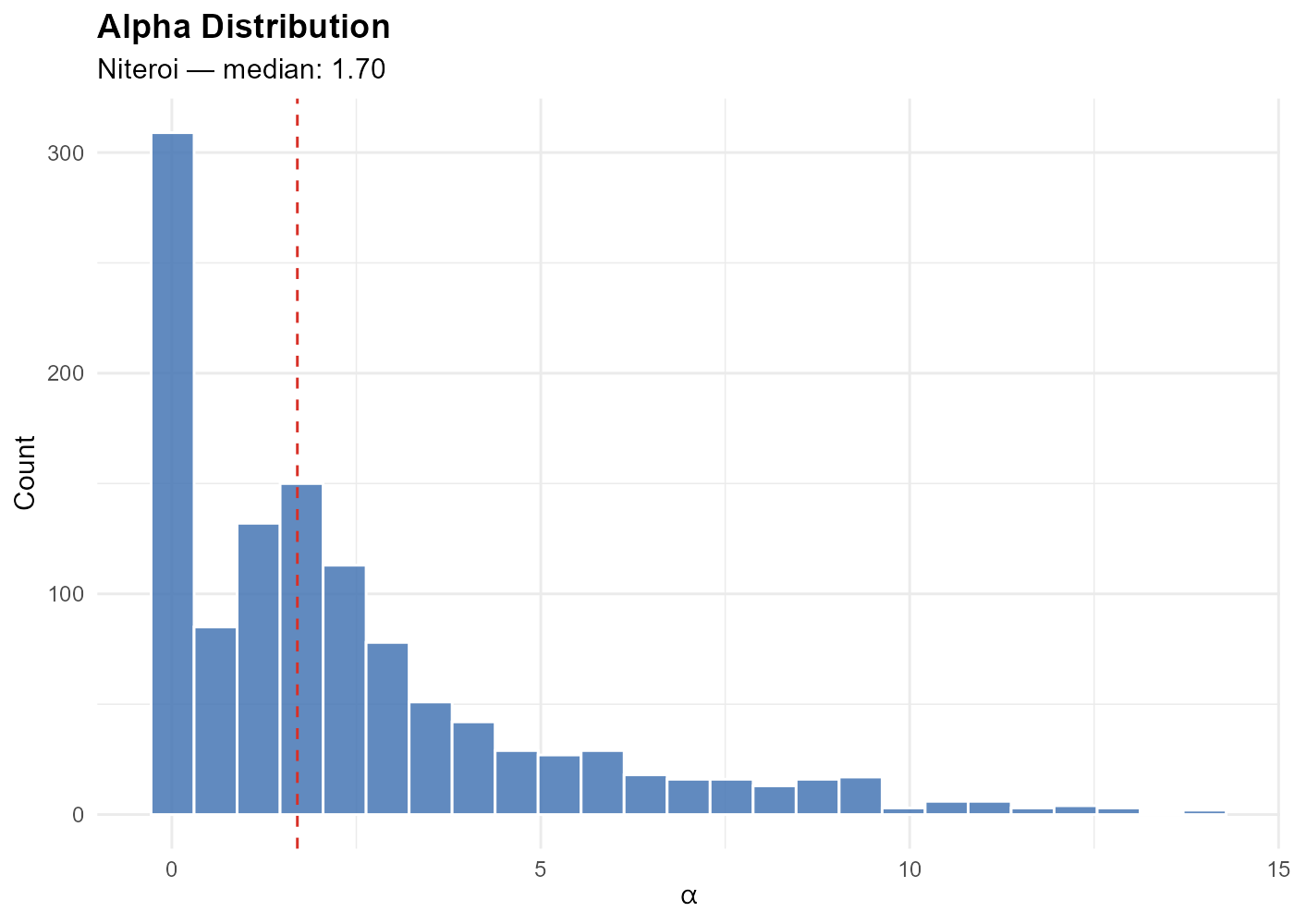
  Alpha:     [0.010, 17.623] (mean 2.507)

The summary() method adds per-variable statistics grouped by type:

summary(result_nit)

The dictionary groups columns by type (candidate, party, turnout, demographics, calibration) with metadata like candidate name, party abbreviation, and ballot number:

View(result_nit$dictionary)

Plotting

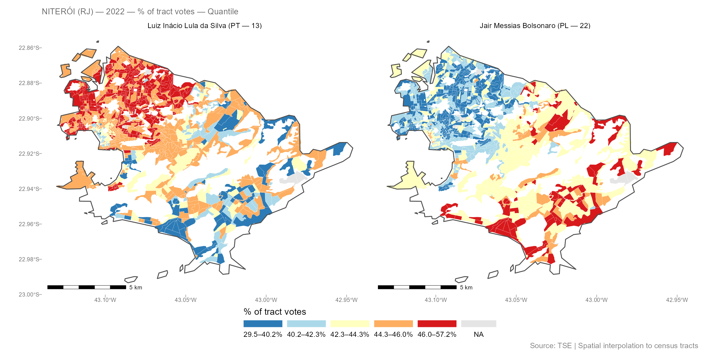
Single variable

plot(result_nit, variable = "Lula")

Variables can be referenced by:

Column name: "CAND_13", "PARTY_PT", "QT_COMPARECIMENTO"
Ballot number: 13, 22
Candidate name (substring, case-insensitive): "Lula", "Bolsonaro"
Party abbreviation: "PT", "PL"

Absolute counts

plot(result_nit, variable = "Lula", type = "absolute")

Faceted comparison

plot(result_nit, variable = c("Lula", "Bolsonaro"), type = "pct_tract")

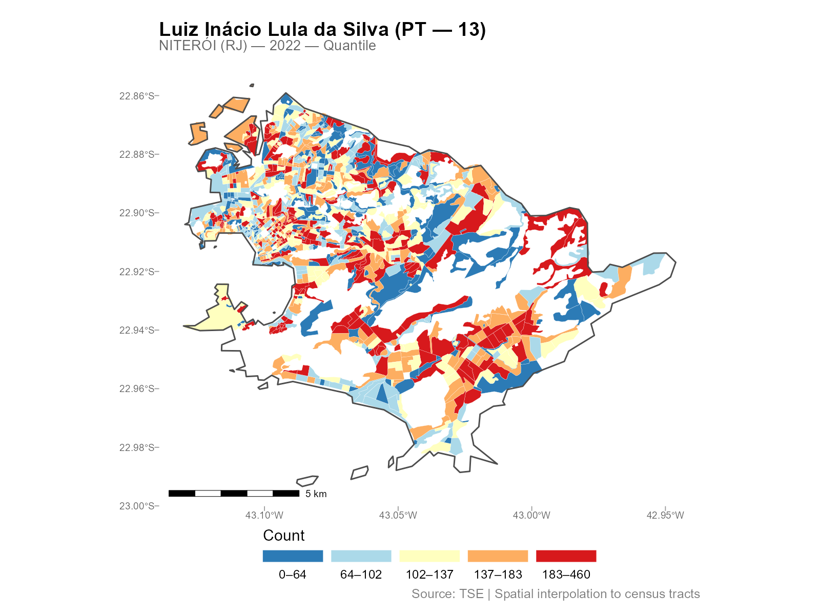
Plot types

The type parameter controls the quantity mapped:

Type	Description
`"pct_tract"`	% of total tract votes (default)
`"absolute"`	Raw interpolated count
`"pct_muni"`	% of municipality total
`"pct_valid"`	% of valid votes (excludes blank/null)
`"pct_eligible"`	% of eligible voters (requires turnout data)
`"density"`	Count per km²

Break methods

The breaks parameter controls the color scale:

"quantile" (default): equal-count bins
"continuous": smooth gradient
"jenks": natural breaks (requires classInt package)
Custom numeric vector: breaks = c(0, 20, 40, 60, 80, 100)

plot(result_nit, variable = "Lula", breaks = "continuous")
plot(result_nit, variable = "Lula", breaks = "jenks")

Additional options

# Overlay polling stations
plot(result_nit, variable = "Lula", show_sources = TRUE)

# Zoom into a region (lon/lat bounding box)
plot(result_nit, variable = "Lula",
     limits = c(-43.15, -43.05, -22.92, -22.86))

# Custom palette
plot(result_nit, variable = "Lula", palette = "viridis")
plot(result_nit, variable = "Lula", palette = "Spectral")

# Composable with ggplot2
library(ggplot2)
plot(result_nit, variable = "Lula") + theme_dark()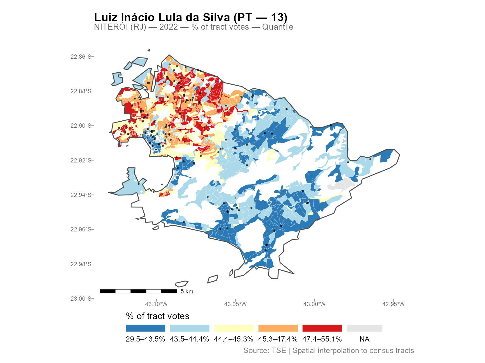

Interactive maps

# Opens in browser with hover tooltips and zoom
plot_interactive(result_nit, variable = "Lula")

Large-scale example (Belo Horizonte)

plot(result_bh, variable = "Lula")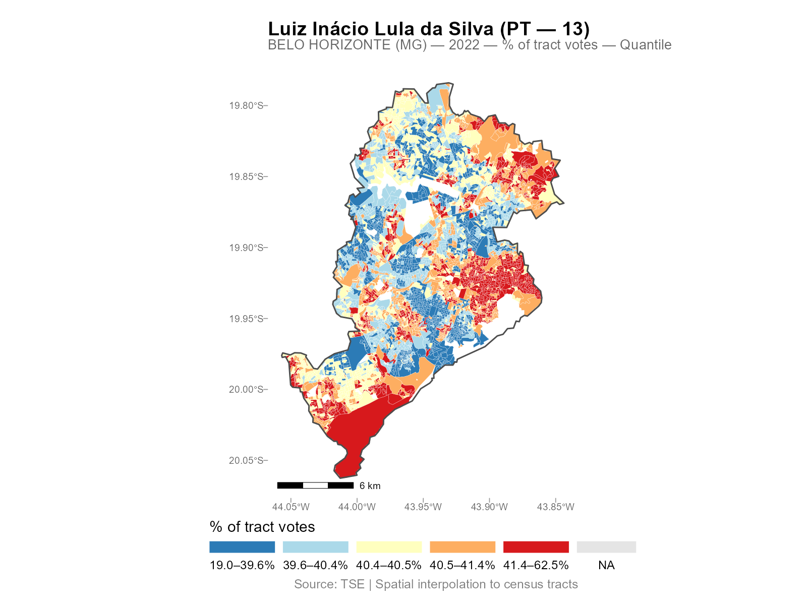

Extracting Alpha

The coef() method returns the optimized decay parameters:

alpha <- coef(result_nit)
summary(alpha)

Map the alpha values spatially to see the urban/peripheral gradient:

result_nit$tracts_sf$alpha <- coef(result_nit)
ggplot(result_nit$tracts_sf) +
  geom_sf(aes(fill = alpha), color = "white", linewidth = 0.05) +
  scale_fill_distiller(palette = "RdYlBu", direction = -1) +
  theme_void()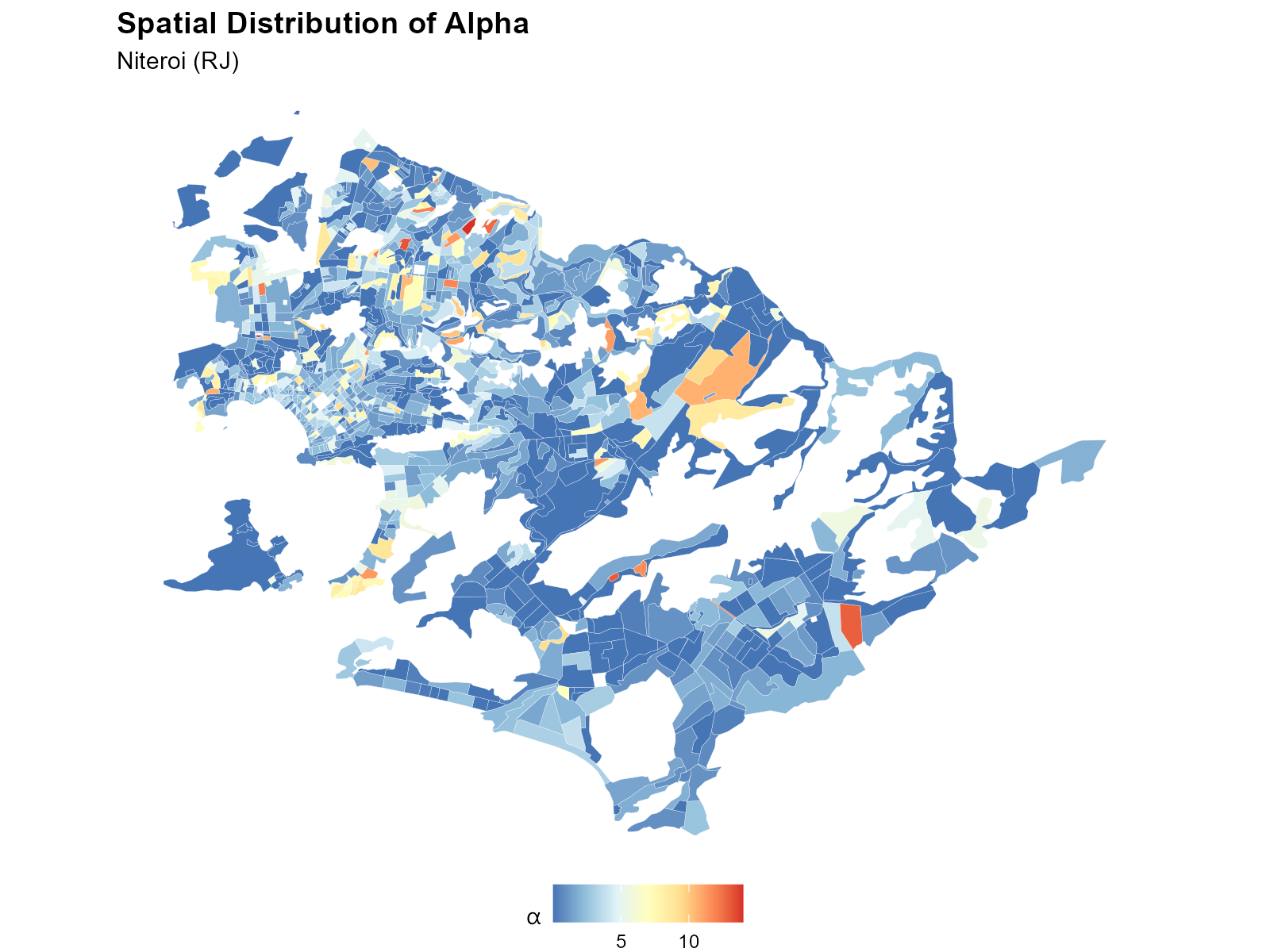

Interpretation: Low alpha (blue) = weight spread across many stations (dense urban areas). High alpha (red) = weight concentrated on the nearest station (periphery).

Residual Analysis

The residuals() method computes the calibration residuals (fitted minus observed) for each tract and age bracket.

resid <- residuals(result_nit)
str(resid)
#> num [1:1169, 1:14] ...

# Per-bracket summary
colMeans(resid)                        # mean residual per bracket
sqrt(colMeans(resid^2))                # RMSE per bracket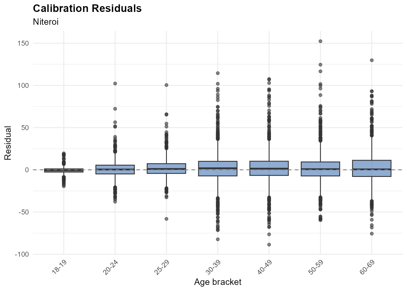

Residuals should be centered near zero. Large residuals may indicate boundary effects (voters crossing municipality borders), data quality issues, or census/election year mismatches.

Validation Checklist

Five checks to apply to any result:

# 1. Total conservation: interpolated totals match source totals
colSums(result_nit$interpolated)[1:3]
colSums(result_nit$sources[, result_nit$interp_cols[1:3]])

# 2. Residual magnitude
resid <- residuals(result_nit)
sqrt(mean(resid^2))   # overall RMSE

# 3. Alpha distribution (no extreme piling at bounds)
summary(coef(result_nit))

# 4. Non-negative values
all(result_nit$interpolated >= -1e-10)

# 5. Convergence
result_nit$optimization$convergence   # 0 = success

Exporting Results

# Plain data frame (no geometry)
df <- as.data.frame(result_nit)
write.csv(df, "niteroi_2022.csv", row.names = FALSE)

# GeoPackage with geometry (for GIS)
sf::st_write(result_nit$tracts_sf, "niteroi_2022.gpkg")

# Column metadata
result_nit$dictionary

# Source-level data (without geometry)
head(result_nit$sources)

The `keep` Parameter

Control which intermediate objects are retained in the result:

Value	Object	Use case
`"weights"`	`result$weights`	`residuals()`, manual reweighting
`"time_matrix"`	`result$time_matrix`	`residuals()` (alternative), reuse
`"electoral_sf"`	`result$electoral_sf`	`plot(..., show_sources = TRUE)`
`"pop_raster"`	`result$pop_raster`	Inspect population density raster
`"rep_points"`	`result$rep_points`	Inspect representative points

weights and time_matrix are always kept by default (needed for residuals() and reinterpolate()). Use keep for additional objects:

result <- interpolate_election_br("Niteroi", year = 2022,
  keep = "electoral_sf")

This also includes source point geometries for overlay plots.