Diagnostics and Validation

interpElections provides 16 diagnostic functions for validating interpolation results. This vignette demonstrates each one using real data from four Brazilian municipalities of varying sizes:

City	State	Tracts	Sources	Character
Igrejinha	RS	~40	~10	Tiny rural municipality
Varginha	MG	~280	~37	Small city (primary example)
Niteroi	RJ	~450	~80	Medium, dense urban area
Belo Horizonte	MG	~5,100	~600	Major metropolitan area

Each section follows the pattern: Intuition (why it matters), Formal definition (the math), Applied example (real output), Interpretation (what to look for).

Setup

library(interpElections)

# Load precomputed results (2022 presidential election)
result_igr  <- readRDS("precomputed/igrejinha_2022.rds")
result_vga  <- readRDS("precomputed/varginha_2022.rds")
result_vga2 <- readRDS("precomputed/varginha_2022_t2.rds")  # turno 2
result_nit  <- readRDS("precomputed/niteroi_2022.rds")
result_bh   <- readRDS("precomputed/belo_horizonte_2022.rds")

Quick overview of each result:

#> interpElections result summary
#> -------------------------------------------------- 
#> Municipality: VARGINHA (MG) -- IBGE: 3170701, TSE: 54135
#> Election: 2022 | Census: 2022 | Turno: 1 | Cargo: PRESIDENTE 
#> Census tracts: 279 | Sources: 37 | Variables: 28
#> 
#> Calibration: gender x 7 age brackets (14 pairs)
#> 
#> Optimization: pb_sgd_colnorm_cpu | Objective: 4670.4370 | Convergence: 0
#>   Alpha: min=1.000, Q1=1.604, median=1.870, Q3=2.227, max=11.836
#> 
#> Candidates (13):
#>   CAND_30                  LUIZ FELIPE CHAVES D AVILA (NOVO) total=        NA  mean=      NA  [NA, NA]
#>   CAND_44                  SORAYA VIEIRA THRONICKE (UNIÃO) total=        NA  mean=      NA  [NA, NA]
#>   CAND_12                  CIRO FERREIRA GOMES (PDT) total=        NA  mean=      NA  [NA, NA]
#>   CAND_13                  LUIZ INÁCIO LULA DA SILVA (PT) total=        NA  mean=      NA  [NA, NA]
#>   ... 9 more -- View(result$dictionary)
#> 
#> Turnout (1):
#>   QT_COMPARECIMENTO        turnout                total=        NA  mean=      NA  [NA, NA]
#> 
#> Calibration (14):
#>   vot_hom_18_19            calibration            total=        NA  mean=      NA  [NA, NA]
#>   vot_hom_20_24            calibration            total=        NA  mean=      NA  [NA, NA]
#>   vot_hom_25_29            calibration            total=        NA  mean=      NA  [NA, NA]
#>   vot_hom_30_39            calibration            total=        NA  mean=      NA  [NA, NA]
#>   vot_hom_40_49            calibration            total=        NA  mean=      NA  [NA, NA]
#>   vot_hom_50_59            calibration            total=        NA  mean=      NA  [NA, NA]
#>   vot_hom_60_69            calibration            total=        NA  mean=      NA  [NA, NA]
#>   vot_mul_18_19            calibration            total=        NA  mean=      NA  [NA, NA]
#>   vot_mul_20_24            calibration            total=        NA  mean=      NA  [NA, NA]
#>   vot_mul_25_29            calibration            total=        NA  mean=      NA  [NA, NA]
#>   vot_mul_30_39            calibration            total=        NA  mean=      NA  [NA, NA]
#>   vot_mul_40_49            calibration            total=        NA  mean=      NA  [NA, NA]
#>   vot_mul_50_59            calibration            total=        NA  mean=      NA  [NA, NA]
#>   vot_mul_60_69            calibration            total=        NA  mean=      NA  [NA, NA]
#> 
#> 
#> Object size: 181.3 MB
#> Neighborhoods: 387

#> interpElections result summary
#> -------------------------------------------------- 
#> Municipality: BELO HORIZONTE (MG) -- IBGE: 3106200, TSE: 41238
#> Election: 2022 | Census: 2022 | Turno: 1 | Cargo: PRESIDENTE 
#> Census tracts: 5109 | Sources: 407 | Variables: 28
#> 
#> Calibration: gender x 7 age brackets (14 pairs)
#> 
#> Optimization: pb_sgd_colnorm_cuda | Objective: 13281.0293 | Convergence: 0
#>   Alpha: min=1.000, Q1=1.248, median=1.357, Q3=1.487, max=17.115
#> 
#> Candidates (13):
#>   CAND_13                  LUIZ INÁCIO LULA DA SILVA (PT) total=    603542  mean=   118.1  [2.8, 334.0]
#>   CAND_27                  JOSE MARIA EYMAEL (DC) total=       209  mean=     0.0  [0.0, 0.3]
#>   CAND_30                  LUIZ FELIPE CHAVES D AVILA (NOVO) total=     14496  mean=     2.8  [0.1, 12.2]
#>   CAND_14                  KELMON LUIS DA SILVA SOUZA (PTB) total=       861  mean=     0.2  [0.0, 1.0]
#>   ... 9 more -- View(result$dictionary)
#> 
#> Turnout (1):
#>   QT_COMPARECIMENTO        turnout                total=   1489578  mean=   291.6  [7.1, 802.2]
#> 
#> Calibration (14):
#>   vot_hom_18_19            calibration            total=     21044  mean=     4.1  [0.0, 12.6]
#>   vot_hom_20_24            calibration            total=     73593  mean=    14.4  [0.3, 44.4]
#>   vot_hom_25_29            calibration            total=     81481  mean=    15.9  [0.4, 58.2]
#>   vot_hom_30_39            calibration            total=    172752  mean=    33.8  [0.8, 102.2]
#>   vot_hom_40_49            calibration            total=    170766  mean=    33.4  [0.8, 113.1]
#>   vot_hom_50_59            calibration            total=    138388  mean=    27.1  [0.7, 71.7]
#>   vot_hom_60_69            calibration            total=    105049  mean=    20.6  [0.4, 52.7]
#>   vot_mul_18_19            calibration            total=     23556  mean=     4.6  [0.0, 15.0]
#>   vot_mul_20_24            calibration            total=     77657  mean=    15.2  [0.3, 46.7]
#>   vot_mul_25_29            calibration            total=     88270  mean=    17.3  [0.4, 69.7]
#>   vot_mul_30_39            calibration            total=    190378  mean=    37.3  [0.9, 110.6]
#>   vot_mul_40_49            calibration            total=    194436  mean=    38.1  [0.9, 136.5]
#>   vot_mul_50_59            calibration            total=    165447  mean=    32.4  [0.8, 86.6]
#>   vot_mul_60_69            calibration            total=    137434  mean=    26.9  [0.6, 68.5]
#> 
#> 
#> Object size: 243.8 MB
#> Neighborhoods: 865

1. Automated Health Check: `diagnostics()`

Intuition

diagnostics() is a single-call “blood test” for your interpolation result. It runs 8 automated checks and reports PASS/WARN/FAIL for each. Use it as a first step after every interpolation to catch problems early.

Only checks whose outcome is not guaranteed by construction are included. Vote conservation, non-negativity, and column normalization are all enforced by design and therefore omitted.

Formal definition

Check	Statistic	PASS	WARN	FAIL
Convergence	Optimizer exit code	code = 0	code != 0	–
Alpha distribution	% of tracts with $\alpha > 15$	< 5%	>= 5%	–
Residual RMSE	$\sqrt{\text{mean}(r^2)}$	always (informational)	–	–
Residual bias	$\max \|\bar{r}_k\| / \text{RMSE}$	ratio < 10%	ratio >= 10%	–
Pop-voter gap	$\|N_{census} - N_{source}\| / \max(N_{census}, N_{source})$	< 5%	5–20%	> 20%
Unreachable pairs	% of $t_{ij}$ near max	< 1%	1–10%	> 10%
Alpha spatial CV	$\text{sd}(\alpha) / \text{mean}(\alpha)$	CV >= 0.1	CV < 0.1	–
Implied turnout	% of tracts with rate > 110%	< 5%	>= 5%	–

Applied example

diagnostics(result_vga)

#> interpElections diagnostics
#> -------------------------------------------------- 
#>  [PASS] Convergence: optimizer converged (code 0)
#>  [PASS] Alpha distribution: median=1.83, IQR=[1.61, 2.16], 0% > 15
#>  [PASS] Residual RMSE: 11.3331 (informational)
#>  [WARN] Residual bias: max |colMeans(resid)| = 8.6344 (76.2% of RMSE)
#>  [WARN] Population-voter gap: census=96829, source=78389, gap=19.0%
#>  [WARN] Unreachable pairs: 2.9% of pairs unreachable (298 / 10323 NA)
#>  [PASS] Alpha spatial variation: CV of median-alpha = 0.492
#>  [PASS] Implied turnout: 1.1% of tracts with implied turnout > 110%
#> -------------------------------------------------- 
#> 5 PASS, 3 WARN

For a larger city:

diagnostics(result_bh)

#> interpElections diagnostics
#> -------------------------------------------------- 
#>  [PASS] Convergence: optimizer converged (code 0)
#>  [PASS] Alpha distribution: median=1.36, IQR=[1.26, 1.47], 0% > 15
#>  [PASS] Residual RMSE: 7.2604 (informational)
#>  [WARN] Residual bias: max |colMeans(resid)| = 1.8894 (26.0% of RMSE)
#>  [PASS] Population-voter gap: census=1650864, source=1640251, gap=0.6%
#>  [FAIL] Unreachable pairs: 48.0% of pairs unreachable (997611 / 2079363 NA)
#>  [PASS] Alpha spatial variation: CV of median-alpha = 0.567
#>  [PASS] Implied turnout: 2.2% of tracts with implied turnout > 110%
#> -------------------------------------------------- 
#> 6 PASS, 1 WARN, 1 FAIL

You can also access check values programmatically:

d <- diagnostics(result_vga, verbose = FALSE)
d$checks$convergence$value
d$checks$residual_rmse$value
d$checks$pop_voter_gap$value

Interpretation

Convergence WARN: The optimizer didn’t converge within the epoch limit. Try increasing max_epochs in optim_control(), or check if the learning rate is too high.
Alpha distribution WARN: Many tracts have very high $\alpha$ values ( $> 15$ ), meaning they effectively use only the nearest station. This can happen when travel time data has poor coverage.
Pop-voter gap WARN/FAIL: The total census population differs substantially from the total registered voters. This is expected to some degree (not everyone registers, some register outside their residence), but gaps > 20% suggest data quality issues.
Unreachable pairs FAIL: Many tract-station pairs have travel times at the ceiling. This means the routing engine couldn’t find paths — check OSM road network coverage.
Alpha spatial CV WARN: Alpha values have very low variation across tracts (CV < 0.1). The optimizer may not be adapting to local conditions, possibly because of insufficient data or poor convergence.

2. Optimization Convergence: `plot_convergence()`

Intuition

The optimizer minimizes Poisson deviance by adjusting the decay parameters $\alpha$ . plot_convergence() shows the optimization trajectory: is the loss decreasing smoothly? Is the gradient approaching zero? What learning rate schedule was used?

Formal definition

Loss: Poisson deviance $= 2 \sum_{i,k} \left[ y_{ik} \log\frac{y_{ik}}{\hat{y}_{ik}} - (y_{ik} - \hat{y}_{ik}) \right]$ , where $y$ = observed census population and $\hat{y}$ = fitted population from the model.
Gradient norm: $\lVert \nabla_\alpha L \rVert_2$ , the Euclidean norm of the gradient of the loss with respect to all alpha parameters.
Learning rate: Step size in gradient descent. May decay over epochs via cosine annealing or other schedules.

Applied examples

All three panels (loss, gradient, learning rate):

plot_convergence(result_vga)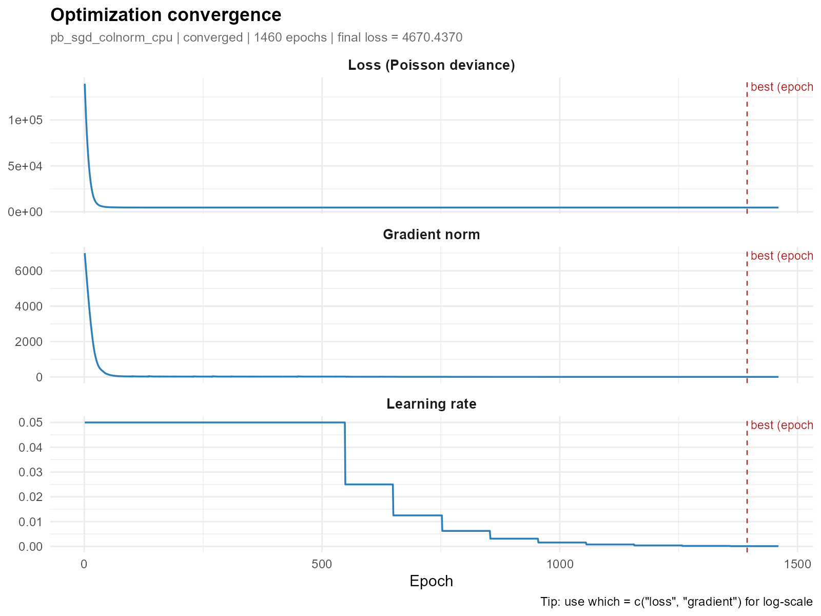

Comparing with a GPU-optimized large city:

plot_convergence(result_bh)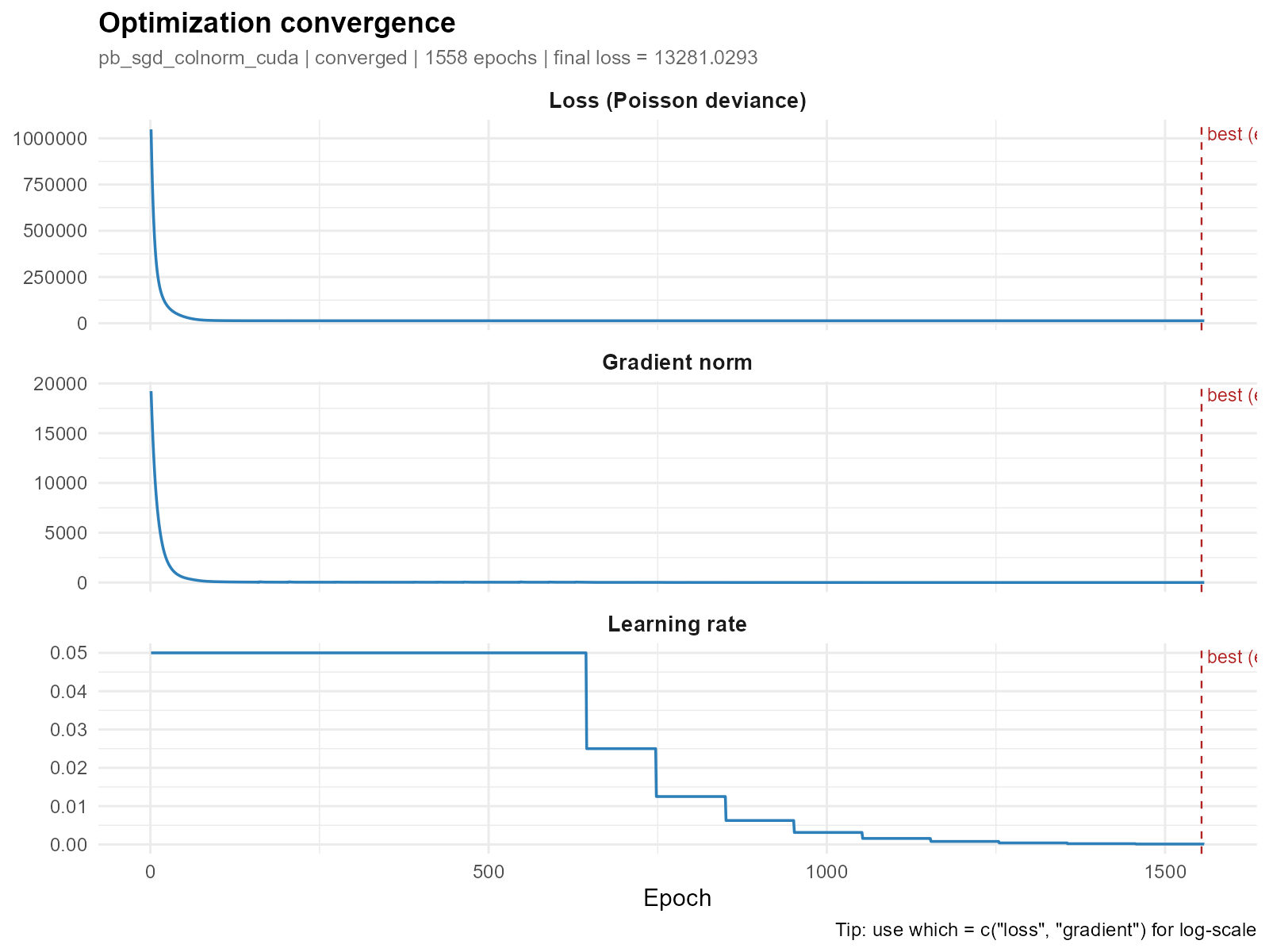

Show only the loss panel:

plot_convergence(result_vga, which = "loss")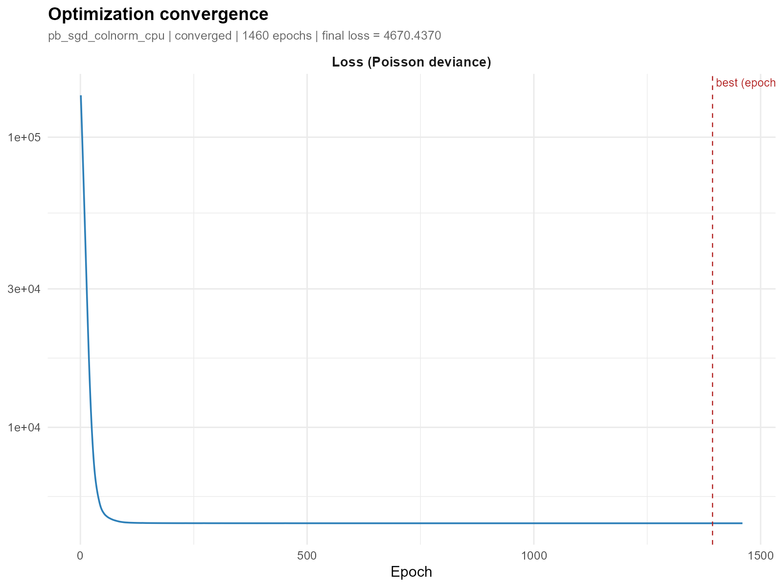

Log scale for loss and gradient (useful when the values span orders of magnitude):

plot_convergence(result_vga, which = c("loss", "gradient"), log_y = TRUE)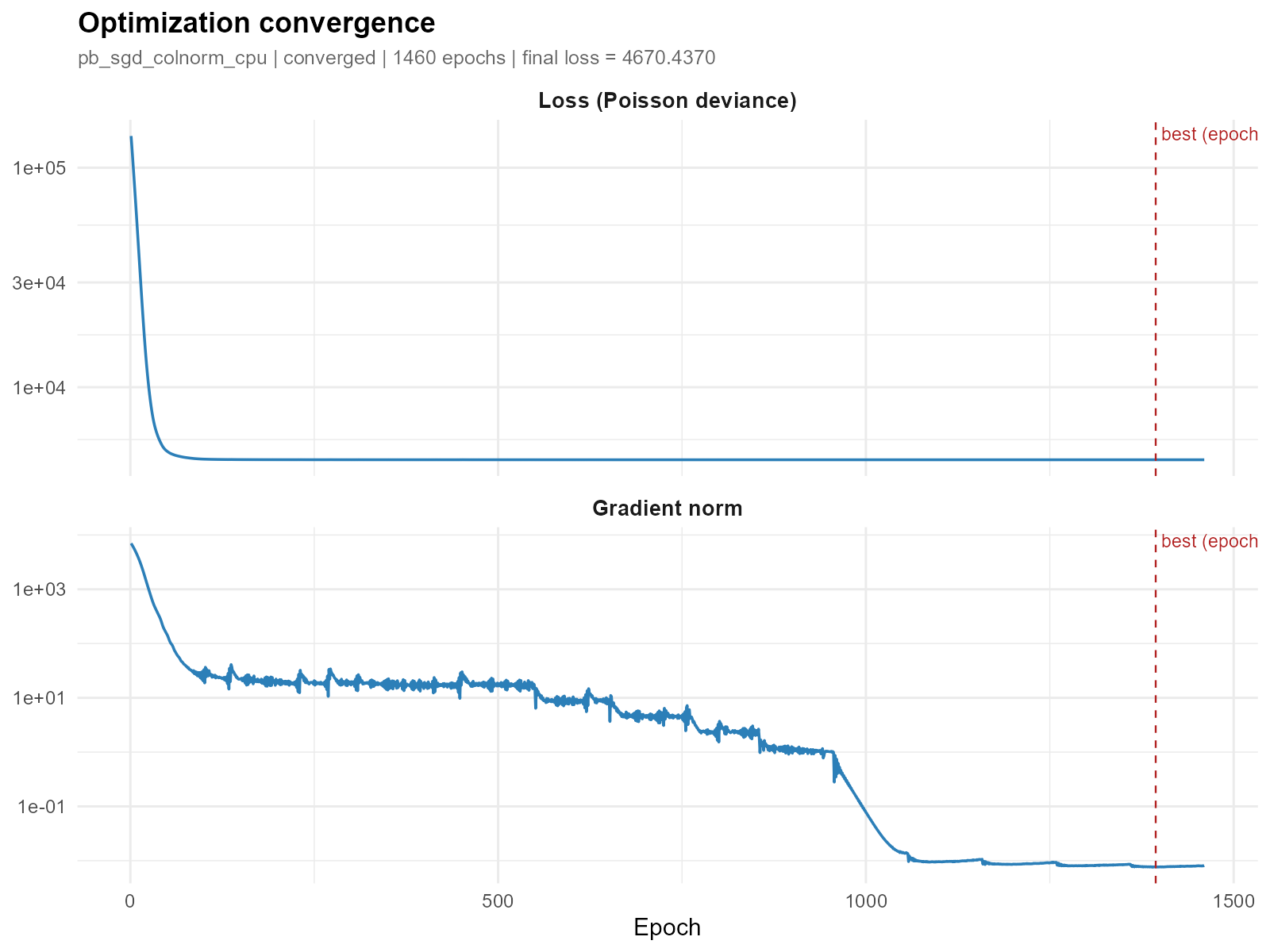

Interpretation

Good convergence: Smooth, monotonically decreasing loss that plateaus. Gradient norm approaches zero. The vertical dashed red line marks the best epoch.
Poor convergence: Oscillating loss, gradient that doesn’t shrink, or loss that hasn’t plateaued by the last epoch. Consider increasing max_epochs or adjusting the learning rate.
Learning rate: The default cosine annealing with warm restarts produces a sawtooth pattern — LR decays to a floor then jumps back up at each restart cycle.

3. Alpha Decay Parameters: `plot_alpha()`

Intuition

The parameter $\alpha_i$ controls how sharply the weight of station $j$ decays with travel time for tract $i$ . Higher $\alpha$ means voters are more localized (sharp decay — only nearby stations matter). Lower $\alpha$ means voters come from a broader area (gradual decay — distant stations still contribute).

$\alpha$ is a matrix with one row per tract and one column per demographic bracket (14 brackets = 7 age groups $\times$ 2 genders). Different brackets may have different decay patterns (e.g., young voters may travel farther to vote).

Formal definition

The weight before column normalization is:

For the default power-law kernel:

$K_{ij} = (t_{ij} + 1)^{-\alpha_i}$

For the exponential kernel (optim_control(kernel = "exponential")):

$K_{ij} = \exp(-\alpha_i \cdot t_{ij})$

The final weight is $W_{ij} = K_{ij} / \sum_i K_{ij}$ (column-normalized so each station’s voters are fully distributed). See vignette("methodology") for details on kernel choice.

Applied examples: Map mode

The map mode collapses the 14-bracket alpha matrix to a single scalar per tract using summary_fn. This is the key visualization choice — different summaries answer different questions.

Median (default) — the “typical” alpha across all brackets:

plot_alpha(result_vga, type = "map", summary_fn = "median")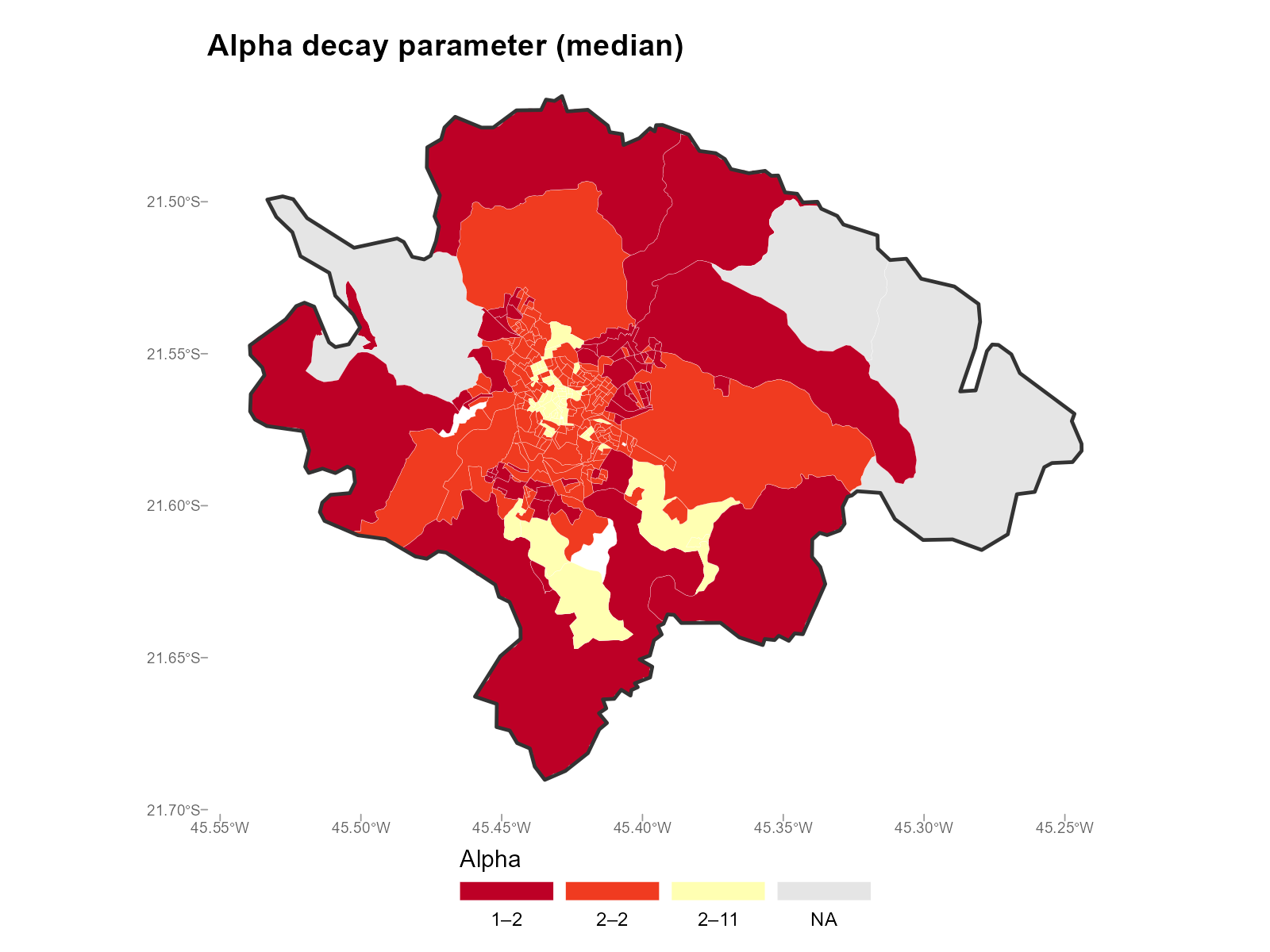

Mean — sensitive to extreme values in any bracket:

plot_alpha(result_vga, type = "map", summary_fn = "mean")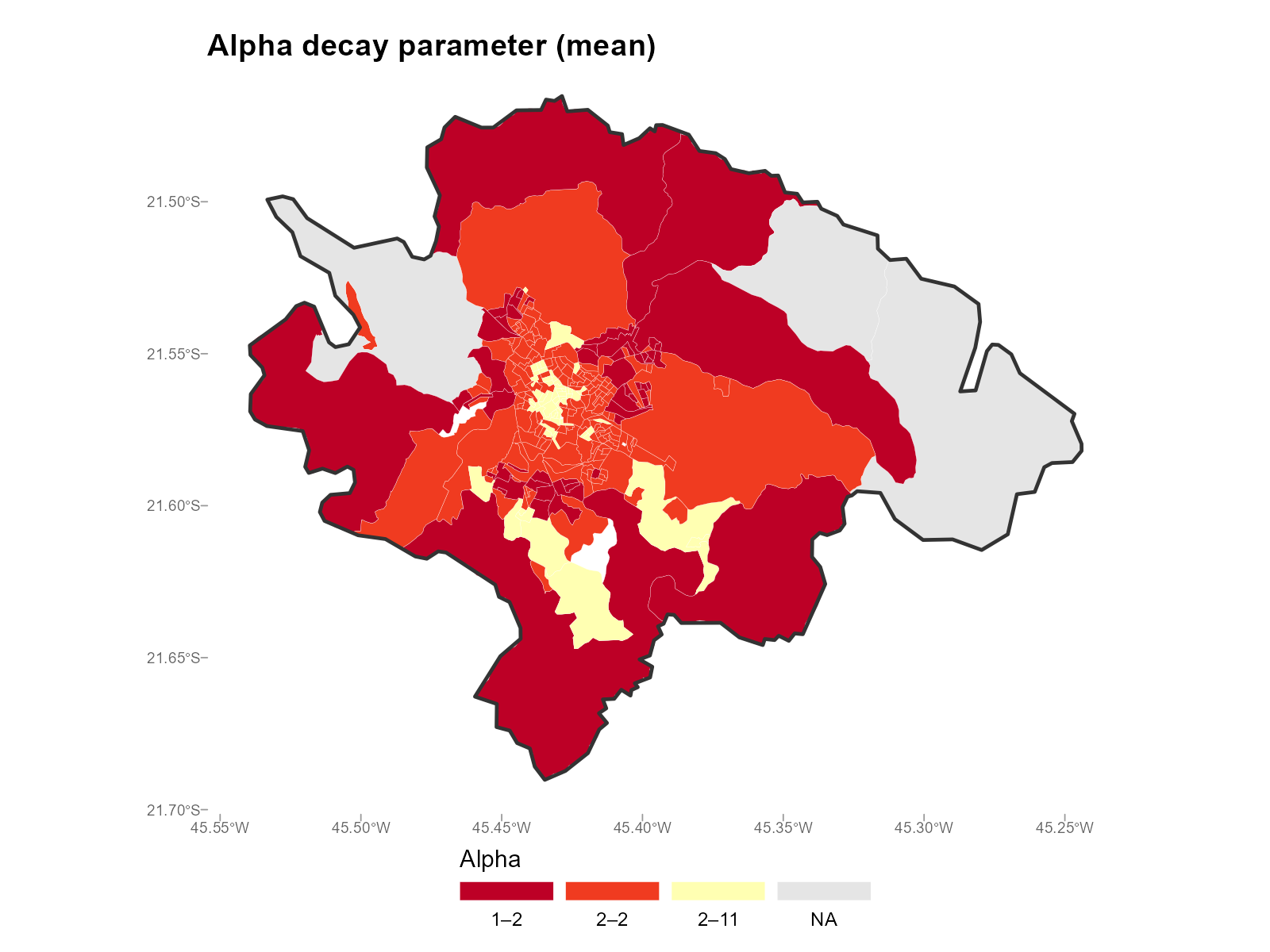

Population-weighted — weights each bracket by the tract’s population in that bracket:

plot_alpha(result_vga, type = "map", summary_fn = "pop_weighted")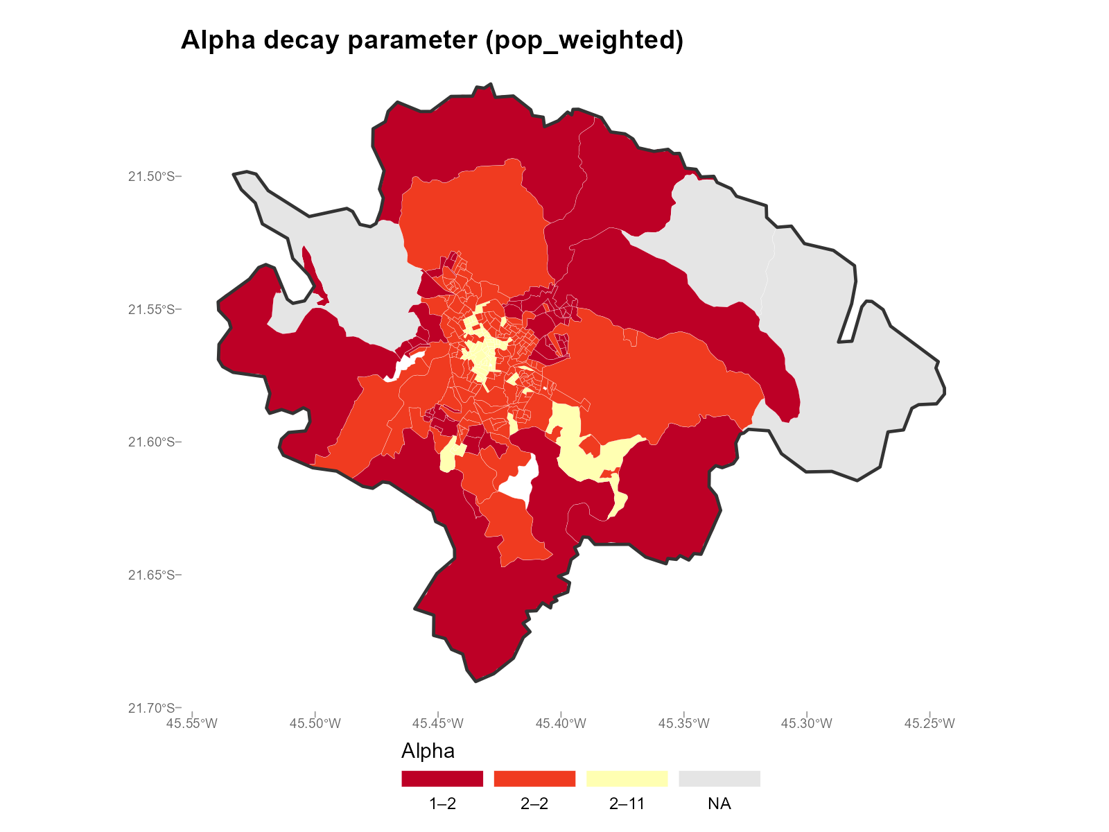

Range ( $\max - \min$ ) — measures how much $\alpha$ varies across brackets within each tract:

plot_alpha(result_vga, type = "map", summary_fn = "range")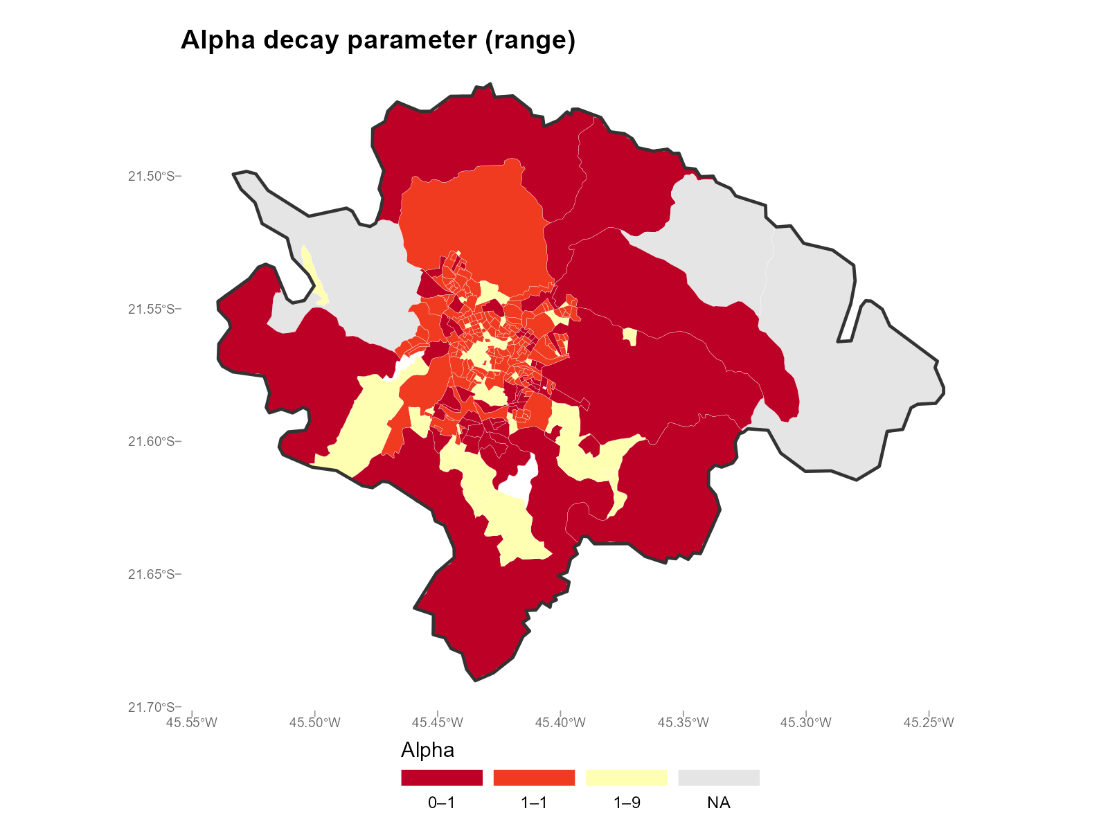

Single bracket (e.g., bracket 1 = Male 18–20):

plot_alpha(result_vga, type = "map", summary_fn = 1)

Large city comparison (Belo Horizonte):

plot_alpha(result_bh, type = "map", summary_fn = "median")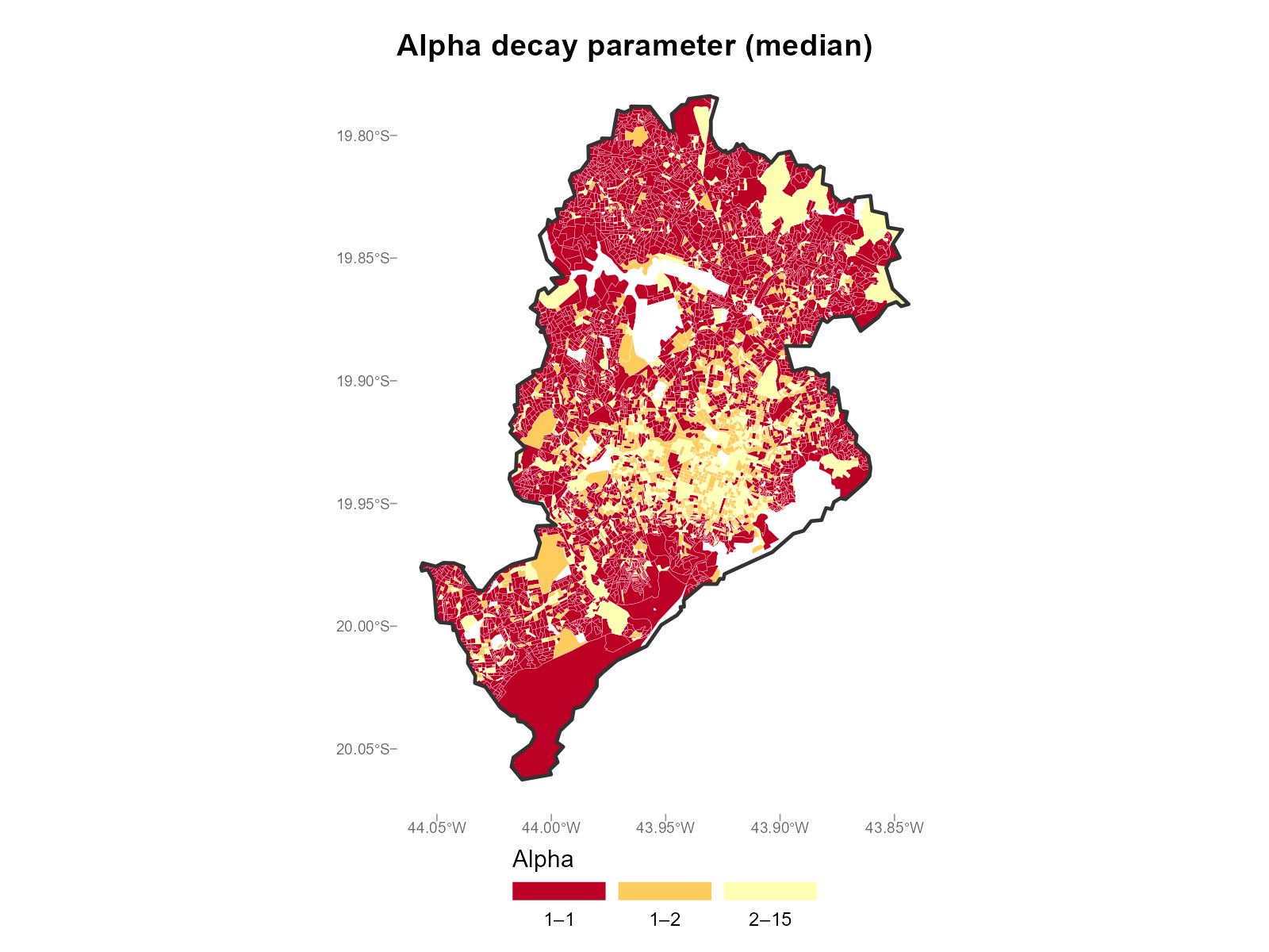

Applied examples: Histogram mode

Density plots faceted by bracket. With 14 brackets arranged in a 2$$7 grid, you can compare age groups and genders at a glance.

plot_alpha(result_nit, type = "histogram")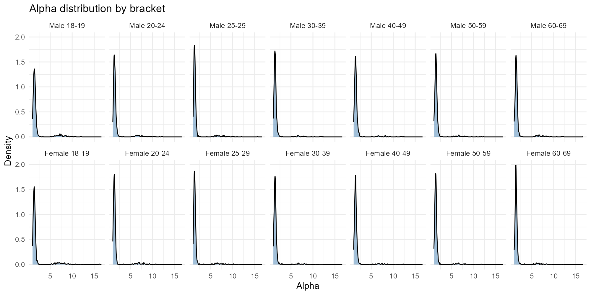

Select specific brackets:

plot_alpha(result_nit, type = "histogram", brackets = c(1, 7, 8, 14))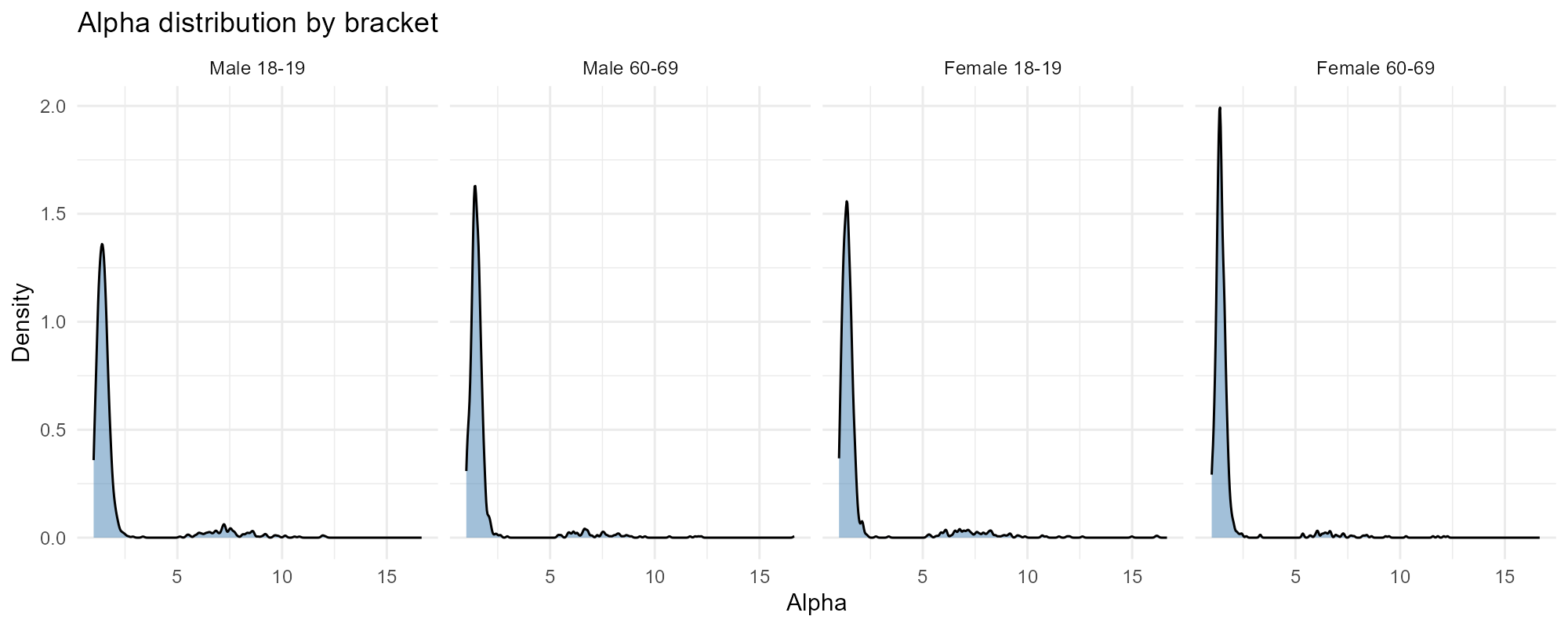

Small city (narrower distributions due to fewer tracts):

plot_alpha(result_igr, type = "histogram")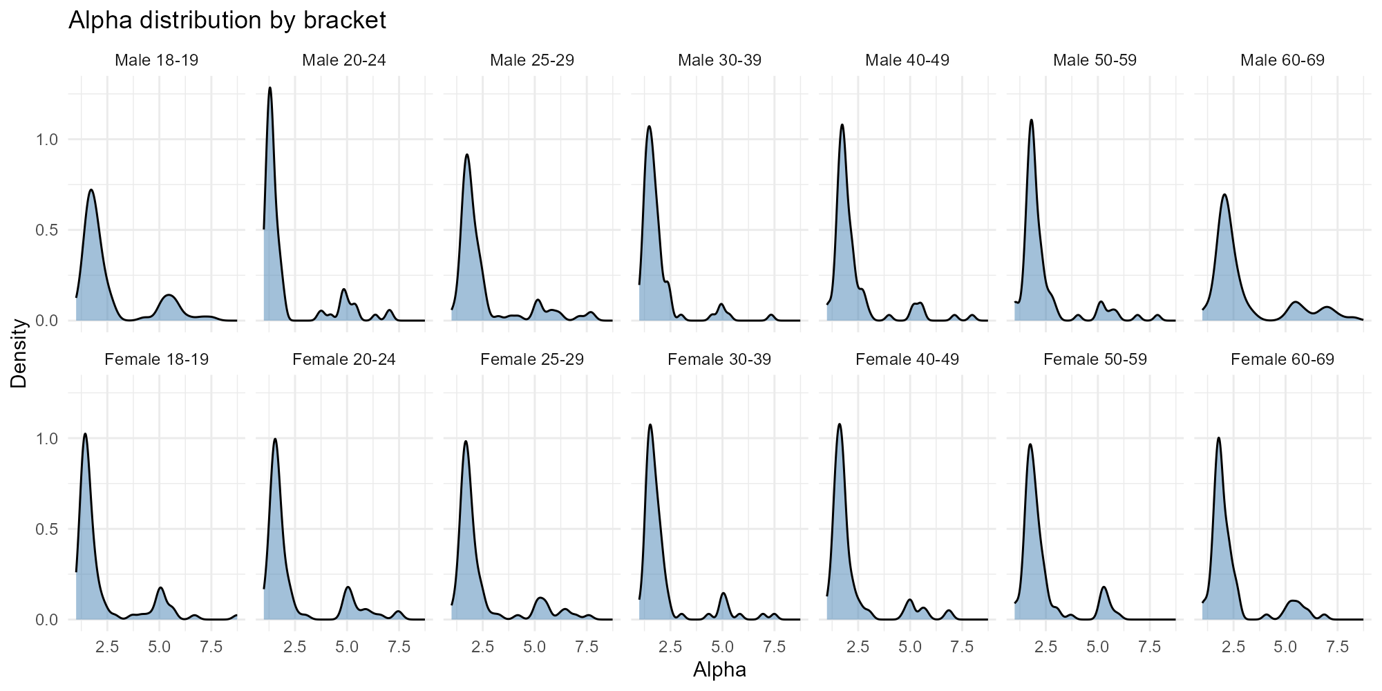

Applied examples: Bracket boxplot

The most compact view — one boxplot per bracket on a single panel:

plot_alpha(result_bh, type = "bracket")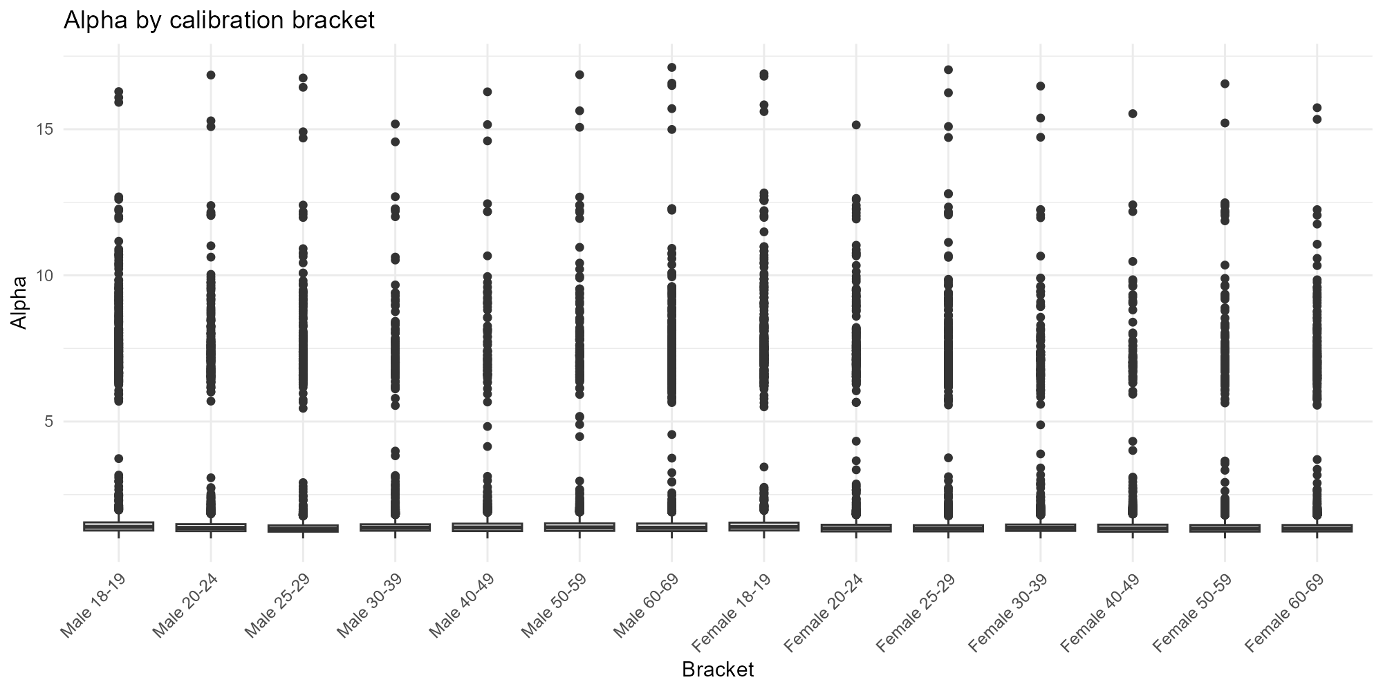

Male brackets only:

plot_alpha(result_nit, type = "bracket", brackets = 1:7)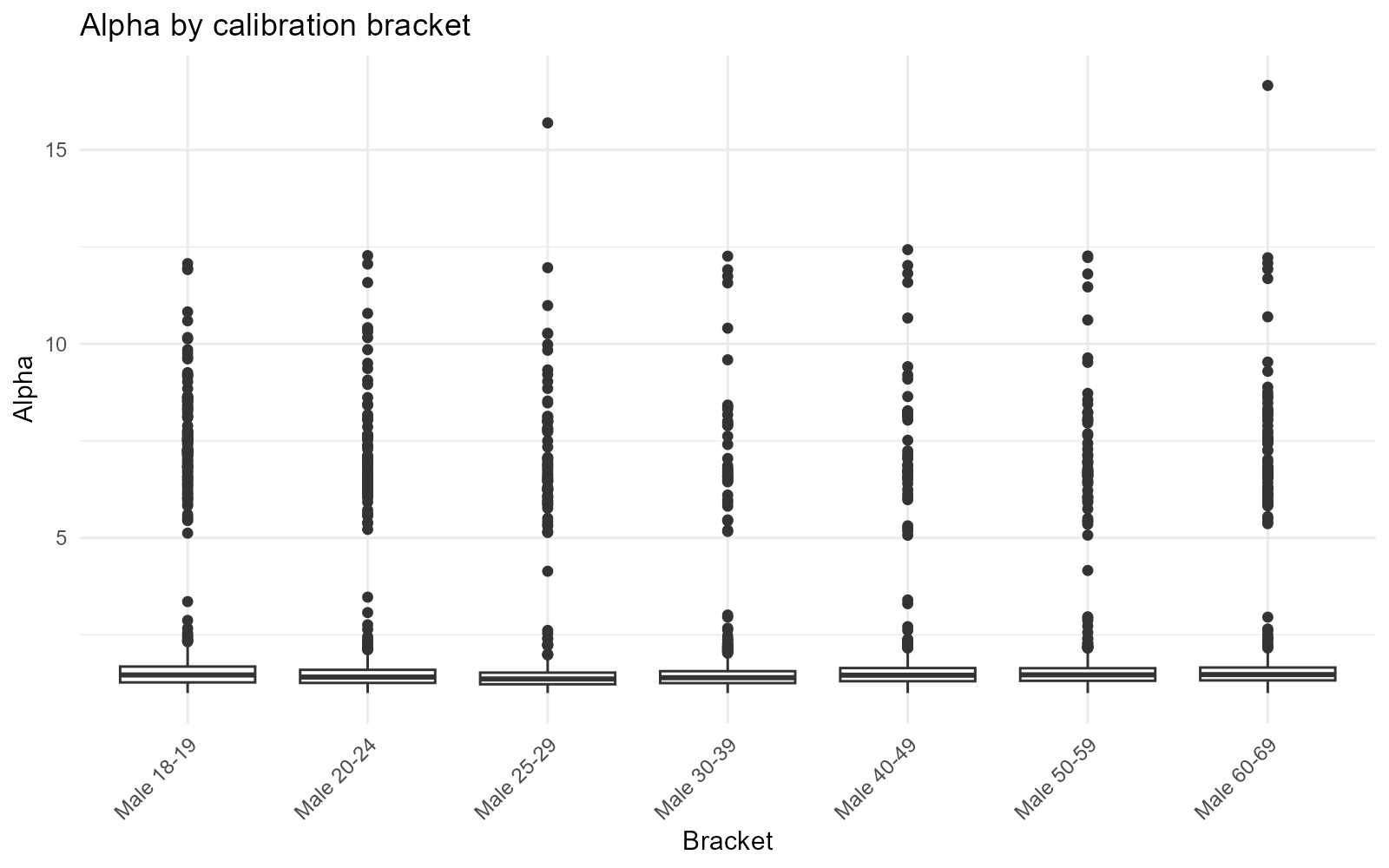

Interpretation

Urban core vs periphery: Central tracts with many nearby stations tend to have higher $\alpha$ (sharper decay). Peripheral tracts with few nearby stations have lower $\alpha$ (they must draw from distant stations).
Age patterns: Younger brackets may show different $\alpha$ distributions than older ones, reflecting different mobility patterns.
Range map: High range = the optimizer found very different decay rates for different brackets in that tract. This often occurs at the urban-rural boundary.
$\alpha > 15$ : Effectively nearest-station assignment. The decay is so steep that only the closest station has non-negligible weight.

4. Calibration Residuals: `plot_residuals()` + `residual_summary()`

Intuition

The model calibrates against known census demographics (population by age $\times$ gender bracket). Residuals measure how well the model reproduces these known quantities. Small residuals mean the model’s spatial allocation of voters closely matches census demographics — giving confidence that the interpolated (unknown) electoral variables are also spatially accurate.

Formal definition

Three types of residuals are available:

Raw: $r_{ik} = \hat{y}_{ik} - y_{ik}$ (fitted minus observed). Scale depends on population size.
Pearson: $r_{ik}^P = (\hat{y}_{ik} - y_{ik}) / \sqrt{\hat{y}_{ik}}$ . Standardized under the Poisson assumption — comparable across tracts of different sizes.
Deviance: $r_{ik}^D = \text{sign}(\hat{y}_{ik} - y_{ik}) \cdot \sqrt{2\left[y_{ik}\log\frac{y_{ik}}{\hat{y}_{ik}} - (y_{ik} - \hat{y}_{ik})\right]}$ . Individual Poisson deviance contributions.

Applied examples: Map mode

For maps, summary_fn collapses across the 14 brackets to a single value per tract.

RMSE (default) — magnitude of misfit:

plot_residuals(result_vga, type = "map", summary_fn = "rmse")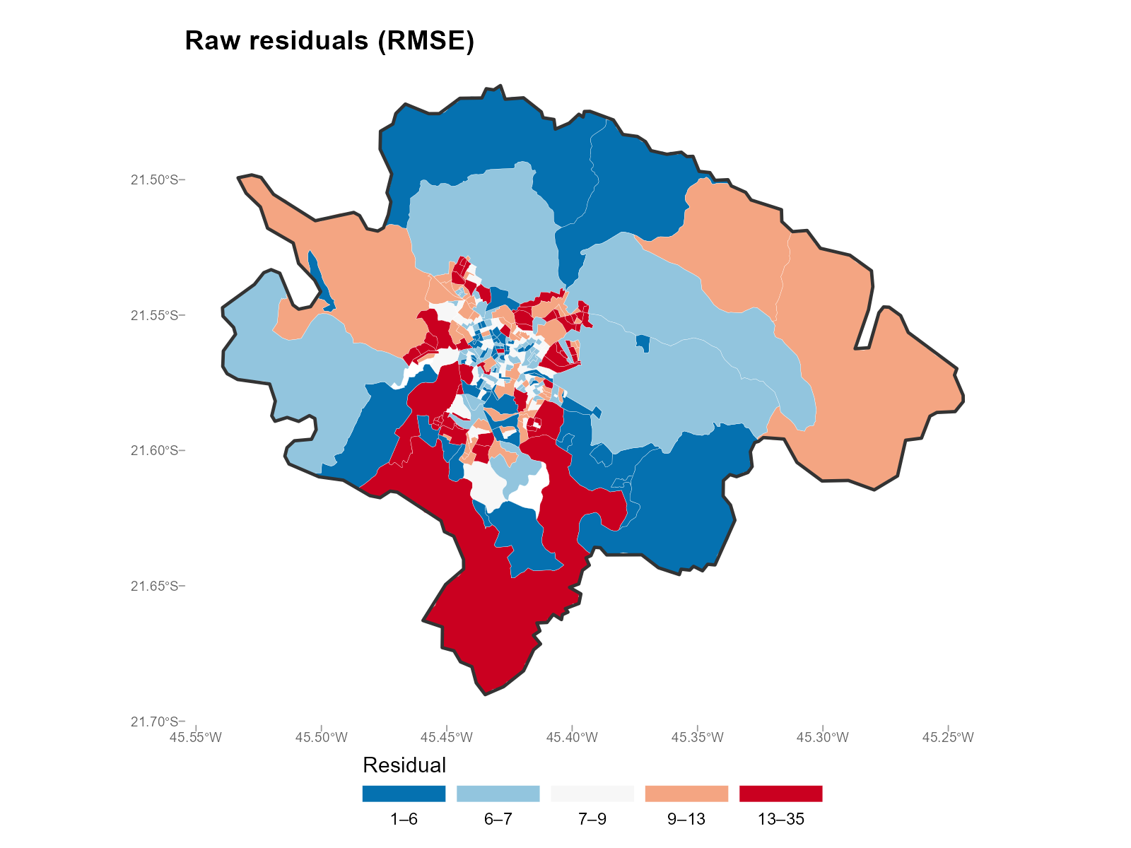

Mean — directional bias (positive = over-prediction, negative = under-prediction):

plot_residuals(result_vga, type = "map", summary_fn = "mean")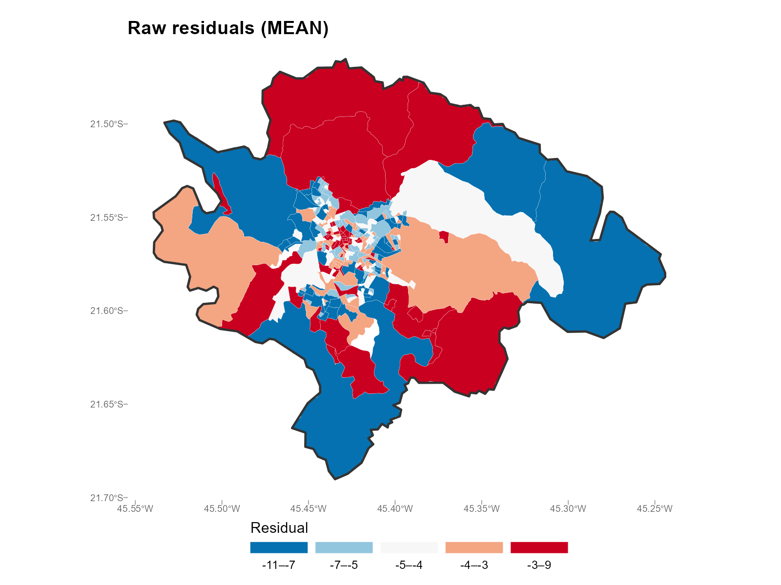

Pearson residuals (standardized):

plot_residuals(result_vga, type = "map", residual_type = "pearson",
               summary_fn = "rmse")

Large city (Belo Horizonte):

plot_residuals(result_bh, type = "map", summary_fn = "rmse")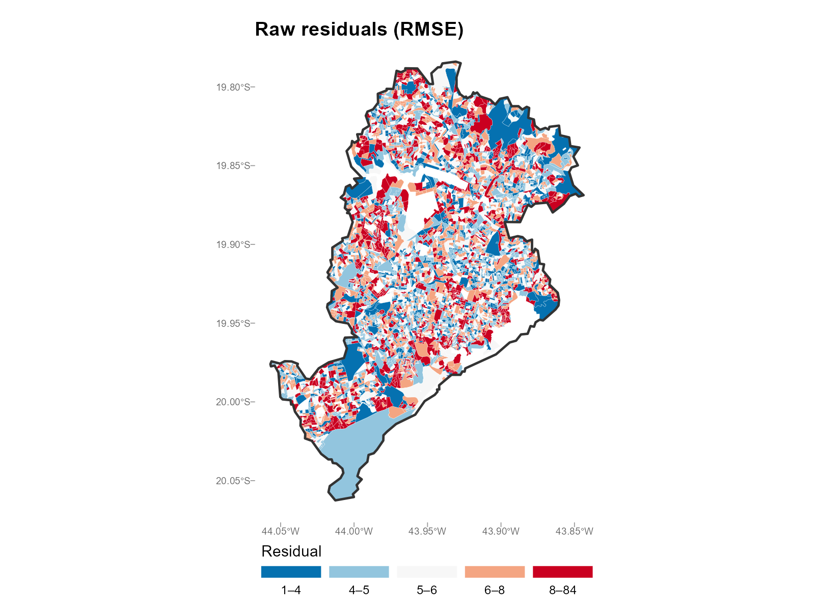

Single bracket:

plot_residuals(result_vga, type = "map", summary_fn = 1)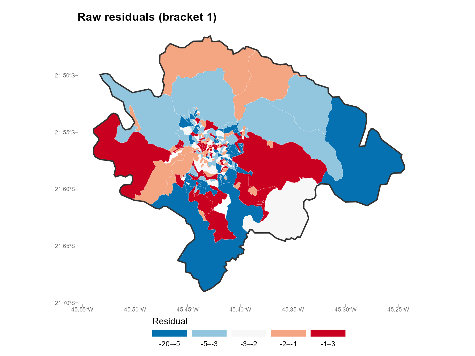

Applied examples: Histogram mode

plot_residuals(result_nit, type = "histogram")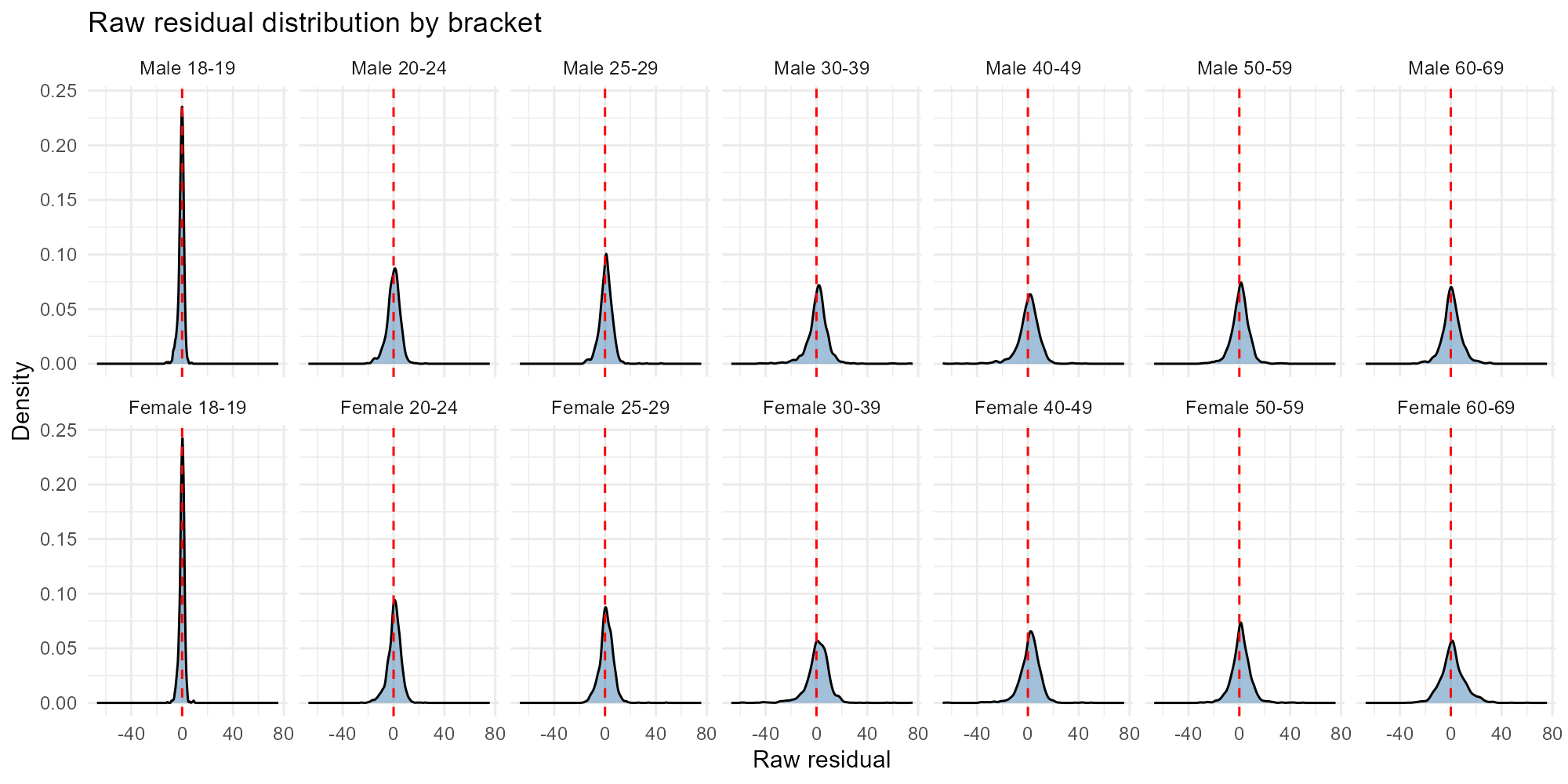

Compare with Pearson residuals:

plot_residuals(result_nit, type = "histogram", residual_type = "pearson")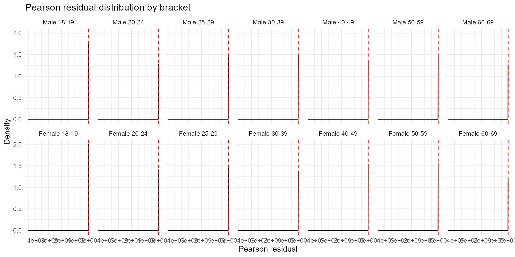

Applied examples: Bracket boxplot

plot_residuals(result_bh, type = "bracket")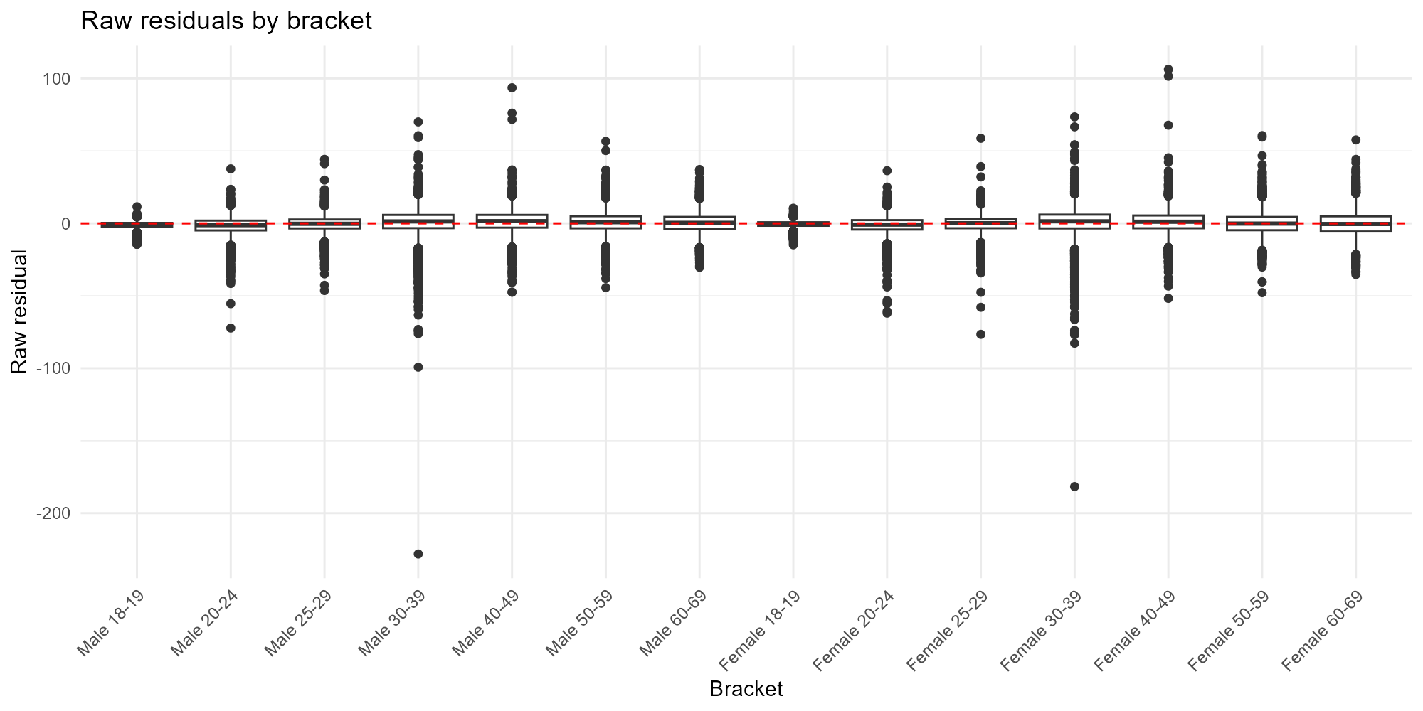

Deviance scale:

plot_residuals(result_bh, type = "bracket", residual_type = "deviance")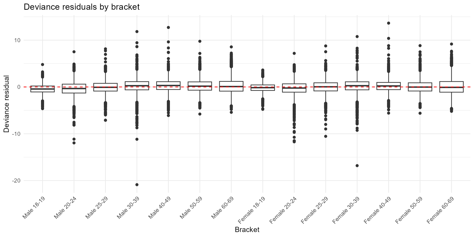

Applied examples: Scatter (fitted vs observed)

plot_residuals(result_igr, type = "scatter")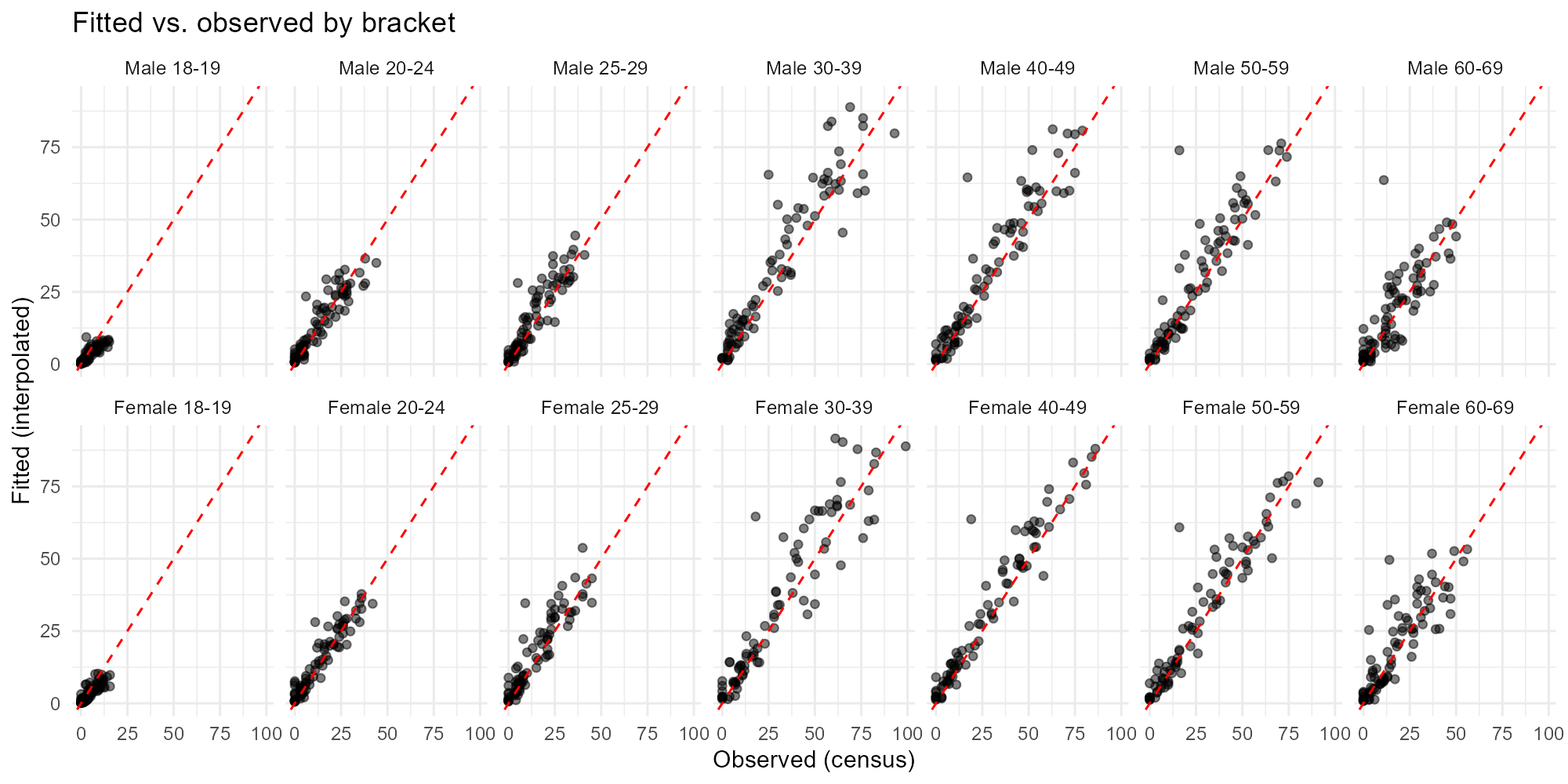

Selected brackets:

plot_residuals(result_vga, type = "scatter", brackets = c(1, 14))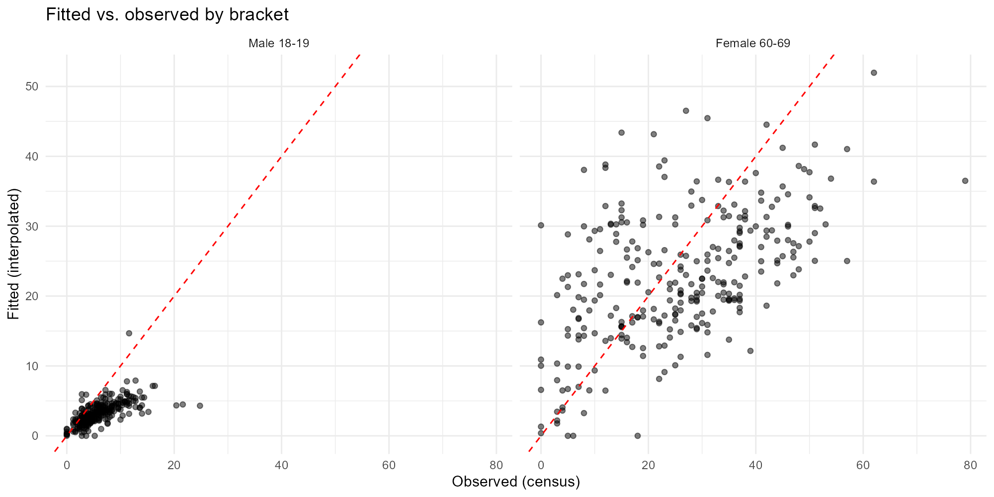

Tabular summary: `residual_summary()`

residual_summary(result_vga)

#> $per_bracket
#>         bracket      mean      rmse  max_abs pct_gt_2sd
#> 1    Male 18-19 -2.827957  4.090797 20.49560  11.111111
#> 2    Male 20-24 -4.939068  7.863136 30.09403  10.752688
#> 3    Male 25-29 -3.688171  8.143861 50.85045   5.376344
#> 4    Male 30-39 -8.189961 17.197483 81.67102   8.243728
#> 5    Male 40-49 -6.788528 12.646651 51.29978   7.885305
#> 6    Male 50-59 -3.684587 10.722865 47.07844   5.734767
#> 7    Male 60-69 -2.093190 10.621665 34.50467   3.942652
#> 8  Female 18-19 -1.896057  3.223661 15.23459   8.243728
#> 9  Female 20-24 -4.594982  8.286037 40.84304   6.451613
#> 10 Female 25-29 -3.767024  9.127714 58.36239   4.659498
#> 11 Female 30-39 -8.634406 18.520190 76.77784   9.318996
#> 12 Female 40-49 -7.537632 13.327423 49.34589  10.035842
#> 13 Female 50-59 -4.498207 11.115594 35.52768   7.526882
#> 14 Female 60-69 -2.953405 12.776099 42.50458   3.584229
#> 
#> $per_tract
#>            tract_id         mean      rmse worst_bracket
#> 1   317070105000001  -4.46978183  7.780279    Male 30-39
#> 2   317070105000008  -5.69532052  6.521208  Female 30-39
#> 3   317070105000009  -6.40664761  9.267085  Female 50-59
#> 4   317070105000010  -4.09593649  8.241522  Female 60-69
#> 5   317070105000013  -5.79583025  7.723394    Male 50-59
#> 6   317070105000014  -4.70288513  6.429955  Female 60-69
#> 7   317070105000015  -3.21996417  5.024781  Female 20-24
#> 8   317070105000016  -3.66598534  5.970083    Male 40-49
#> 9   317070105000017  -8.02832181 10.453555  Female 30-39
#> 10  317070105000019  -3.39119823  5.524819    Male 60-69
#> 11  317070105000021  -5.09111145  7.203794    Male 40-49
#> 12  317070105000022  -2.92625683  5.141192  Female 25-29
#> 13  317070105000023  -4.70994909  7.473714    Male 30-39
#> 14  317070105000024  -4.65966836  7.084826    Male 25-29
#> 15  317070105000025  -3.58820938  7.515399  Female 60-69
#> 16  317070105000026  -2.59066838  4.599541  Female 30-39
#> 17  317070105000028  -7.85698397 15.446466  Female 30-39
#> 18  317070105000029  -5.40849541  8.450547  Female 40-49
#> 19  317070105000031  -3.89397077  5.834789  Female 60-69
#> 20  317070105000032  -5.28109306  8.720115    Male 20-24
#> 21  317070105000033  -3.80484335  5.778048    Male 60-69
#> 22  317070105000035  -4.22505171  6.261096  Female 30-39
#> 23  317070105000036  -5.25458948  9.366690    Male 30-39
#> 24  317070105000037  -3.69797455  5.705231  Female 60-69
#> 25  317070105000039  -5.18900581  7.768118    Male 40-49
#> 26  317070105000040  -5.54970207 17.902995    Male 50-59
#> 27  317070105000041  -4.35580469  8.416798  Female 50-59
#> 28  317070105000043  -2.92924034  5.086059    Male 40-49
#> 29  317070105000044  -4.92242984 14.221143    Male 40-49
#> 30  317070105000045  -5.54451610  9.378096  Female 40-49
#> 31  317070105000047  -6.87290218 11.932898  Female 50-59
#> 32  317070105000048  -4.12777463  7.548253    Male 30-39
#> 33  317070105000049  -3.86660142  5.565906  Female 30-39
#> 34  317070105000050  -5.07588214  8.838433  Female 60-69
#> 35  317070105000051  -3.16488998  4.579301  Female 40-49
#> 36  317070105000052  -4.98188243  7.269529  Female 30-39
#> 37  317070105000054  -4.35382028  8.647110  Female 60-69
#> 38  317070105000055  -4.29991404 11.477892  Female 50-59
#> 39  317070105000056  -2.65074687  5.708509  Female 60-69
#> 40  317070105000057  -3.53921237  7.376684  Female 60-69
#> 41  317070105000059  -5.54329305  8.078800  Female 40-49
#> 42  317070105000060  -5.67776673  7.052883    Male 50-59
#> 43  317070105000061  -4.54991476  6.796096  Female 50-59
#> 44  317070105000063  -4.27955069  9.015014  Female 60-69
#> 45  317070105000065  -6.46841403  9.618279    Male 60-69
#> 46  317070105000066  -5.61921541 11.229709    Male 60-69
#> 47  317070105000067  -3.70455425  7.798223  Female 50-59
#> 48  317070105000069  -7.08697385  9.610891    Male 30-39
#> 49  317070105000070  -5.11650942  8.360278  Female 50-59
#> 50  317070105000071  -5.00843229  7.873160  Female 60-69
#> 51  317070105000074  -4.61650515  7.532968  Female 60-69
#> 52  317070105000077  -3.93589804  9.000784  Female 60-69
#> 53  317070105000078  -5.27064515  8.735191  Female 60-69
#> 54  317070105000079  -5.42014183  8.153125  Female 40-49
#> 55  317070105000082  -5.65931668  8.814523    Male 60-69
#> 56  317070105000083  -4.67848798  8.477325  Female 50-59
#> 57  317070105000086  -5.79974066  9.232188    Male 40-49
#> 58  317070105000087  -5.33495329  8.472898  Female 50-59
#> 59  317070105000089  -7.47620551 10.905327  Female 40-49
#> 60  317070105000091  -5.88057711  9.118924  Female 60-69
#> 61  317070105000094  -6.92574008  9.256367  Female 60-69
#> 62  317070105000095  -7.06021306  9.379119    Male 40-49
#> 63  317070105000096  -6.87335323 10.553908  Female 40-49
#> 64  317070105000100  -9.94300685 15.623448  Female 40-49
#> 65  317070105000101  -4.73015509  8.957741    Male 50-59
#> 66  317070105000102  -9.45775086 14.596251  Female 50-59
#> 67  317070105000103  -3.42464735  6.877452  Female 60-69
#> 68  317070105000104  -5.05947052 10.247530  Female 60-69
#> 69  317070105000105  -6.64221452 10.466741  Female 60-69
#> 70  317070105000106  -4.74402852  7.739311  Female 60-69
#> 71  317070105000107  -5.04264300  9.476863  Female 60-69
#> 72  317070105000108  -4.52430196 11.836652  Female 60-69
#> 73  317070105000112 -10.70524209 19.208083  Female 40-49
#> 74  317070105000114  -7.58292592 12.414566  Female 50-59
#> 75  317070105000115  -7.85118226 12.988053    Male 50-59
#> 76  317070105000116  -5.23164076 10.780131    Male 50-59
#> 77  317070105000117  -5.95415250  9.466325  Female 40-49
#> 78  317070105000120  -4.89691516 14.875840  Female 30-39
#> 79  317070105000121  -1.44764559  5.226840    Male 50-59
#> 80  317070105000124  -9.30533133 12.488768  Female 30-39
#> 81  317070105000125  -7.83185485  9.944685  Female 40-49
#> 82  317070105000126  -4.28045952  6.748654  Female 60-69
#> 83  317070105000127  -4.77031584  7.512045  Female 50-59
#> 84  317070105000128  -6.51097071 10.078242    Male 60-69
#> 85  317070105000129  -5.90250621  9.063544  Female 50-59
#> 86  317070105000130  -5.64954139  6.886282  Female 50-59
#> 87  317070105000131  -6.75248864 12.220189  Female 60-69
#> 88  317070105000133  -6.03865184 13.555790  Female 60-69
#> 89  317070105000134  -3.08150406  6.888872  Female 50-59
#> 90  317070105000135  -4.89329067  9.373227  Female 60-69
#> 91  317070105000136  -1.84728816  5.654837  Female 30-39
#> 92  317070105000138 -11.01428571 12.405644  Female 60-69
#> 93  317070105000139  -2.83529955  7.100915    Male 50-59
#> 94  317070105000140  -1.73322996  5.343345    Male 50-59
#> 95  317070105000141  -1.96477361  4.927858    Male 50-59
#> 96  317070105000142 -10.51428571 12.016417    Male 40-49
#> 97  317070105000143 -10.95714286 12.349320  Female 40-49
#> 98  317070105000144  -4.29576738  6.475777    Male 40-49
#> 99  317070105000147  -7.57497684 13.883793    Male 40-49
#> 100 317070105000148  -6.95230788  9.746854  Female 40-49
#> 101 317070105000149  -4.04310841  9.315555  Female 50-59
#> 102 317070105000150  -0.09205360  2.453728  Female 60-69
#> 103 317070105000151  -9.38574168 14.562069    Male 50-59
#> 104 317070105000152  -4.05701272 10.191480  Female 60-69
#> 105 317070105000153  -5.12329326  7.086856  Female 60-69
#> 106 317070105000154  -5.97116573  7.561613  Female 50-59
#> 107 317070105000155  -4.40479715  5.876291  Female 50-59
#> 108 317070105000156  -3.38121653  6.447234  Female 60-69
#> 109 317070105000157  -7.38748886 14.083776  Female 40-49
#> 110 317070105000158  -4.51901512  6.005070    Male 60-69
#> 111 317070105000159  -6.55120159 15.163124  Female 40-49
#> 112 317070105000160  -5.82683227 10.990449  Female 50-59
#> 113 317070105000161  -8.37639883 13.662417  Female 50-59
#> 114 317070105000162  -6.40080059 13.818299    Male 50-59
#> 115 317070105000164  -2.37118808  8.546970  Female 30-39
#> 116 317070105000165   0.22212169  1.101596  Female 25-29
#> 117 317070105000166  -6.87200698  9.183925  Female 50-59
#> 118 317070105000168  -7.55816260  9.901026  Female 40-49
#> 119 317070105000169  -6.18064683  8.358678  Female 60-69
#> 120 317070105000171  -5.65975764 14.035889  Female 40-49
#> 121 317070105000172  -5.31781160 16.142278    Male 40-49
#> 122 317070105000174  -4.72435992 16.356485    Male 30-39
#> 123 317070105000175  -2.71496952 10.298496  Female 30-39
#> 124 317070105000176  -1.55969492  3.617670  Female 30-39
#> 125 317070105000177   9.37303532 14.054435  Female 30-39
#> 126 317070105000178  -4.56211561 14.353457  Female 30-39
#> 127 317070105000179  -4.06906832  6.673661  Female 60-69
#> 128 317070105000180  -3.81645096  6.853486  Female 60-69
#> 129 317070105000181  -3.05099036  6.596282    Male 60-69
#> 130 317070105000182  -6.13905913 19.792027  Female 30-39
#> 131 317070105000183  -9.32212146 19.624818  Female 40-49
#> 132 317070105000185  -4.35020716  6.326250  Female 50-59
#> 133 317070105000186  -4.26238139  8.832778  Female 60-69
#> 134 317070105000188  -7.11605725  9.998682  Female 40-49
#> 135 317070105000189  -4.48957226  8.247922  Female 60-69
#> 136 317070105000190  -3.48081790  4.948018  Female 40-49
#> 137 317070105000191  -2.16225685  5.348972  Female 60-69
#> 138 317070105000192  -3.98062714  7.363546  Female 30-39
#> 139 317070105000193  -3.41123408  8.592075    Male 30-39
#> 140 317070105000194  -5.89246770 10.087114    Male 20-24
#> 141 317070105000196  -7.41453811 23.364285  Female 30-39
#> 142 317070105000197   0.08298607  1.586720    Male 30-39
#> 143 317070105000198  -0.52907993  1.760266    Male 60-69
#> 144 317070105000199  -5.66189173  9.579314  Female 40-49
#> 145 317070105000200  -7.39849787 13.993152    Male 40-49
#> 146 317070105000201  -7.37047749 13.272088  Female 50-59
#> 147 317070105000205  -7.30761777 20.104961  Female 40-49
#> 148 317070105000206  -7.38316109 18.697316  Female 40-49
#> 149 317070105000207  -2.19033493  6.801264    Male 20-24
#> 150 317070105000208  -5.74515367 15.286066  Female 30-39
#> 151 317070105000209  -7.17987136 18.356939  Female 30-39
#> 152 317070105000210  -5.18184771 12.734001  Female 40-49
#> 153 317070105000211  -3.76001088 11.339685  Female 40-49
#> 154 317070105000212  -4.63035739 11.521751  Female 40-49
#> 155 317070105000213  -5.17376113 13.426430  Female 30-39
#> 156 317070105000214  -8.88049176 26.172918  Female 30-39
#> 157 317070105000216  -6.60765474 20.959614    Male 30-39
#> 158 317070105000217  -2.98070111 11.574437  Female 30-39
#> 159 317070105000219  -9.00126981 30.011366    Male 30-39
#> 160 317070105000220  -2.24084214  6.325360    Male 20-24
#> 161 317070105000221  -3.40950336  6.094611  Female 60-69
#> 162 317070105000222  -2.09463879  4.456393    Male 60-69
#> 163 317070105000223  -1.54964403  4.448766  Female 60-69
#> 164 317070105000224  -2.54114135  7.189218  Female 25-29
#> 165 317070105000225  -2.06761302  5.207428    Male 60-69
#> 166 317070105000226  -2.03412647  4.494774    Male 25-29
#> 167 317070105000227  -3.93916279  7.105443    Male 30-39
#> 168 317070105000228  -2.88029353  4.856285  Female 20-24
#> 169 317070105000229  -3.72300315  6.301937  Female 60-69
#> 170 317070105000230  -3.40944562  4.990152  Female 60-69
#> 171 317070105000231  -3.85189135  6.035891    Male 30-39
#> 172 317070105000232  -2.85902328  4.248717    Male 60-69
#> 173 317070105000233  -2.60761506  3.980579    Male 30-39
#> 174 317070105000234  -2.04350410  4.884697    Male 20-24
#> 175 317070105000235  -3.92571869  6.701134  Female 30-39
#> 176 317070105000236  -2.29353158  4.713671  Female 20-24
#> 177 317070105000237  -5.05134358  8.760045  Female 40-49
#> 178 317070105000238  -3.10664216  6.845682  Female 60-69
#> 179 317070105000239  -2.58490714  4.991092  Female 50-59
#> 180 317070105000240  -2.55276300  5.017651  Female 60-69
#> 181 317070105000241  -3.29748551  9.692393  Female 50-59
#> 182 317070105000242  -5.47205505  8.967630    Male 30-39
#> 183 317070105000243  -2.94082344  5.089976    Male 30-39
#> 184 317070105000244  -2.92593525  5.871260    Male 20-24
#> 185 317070105000245  -6.09796927  7.880939  Female 40-49
#> 186 317070105000246  -4.79644059 14.507438  Female 30-39
#> 187 317070105000247  -3.87800652  5.314640    Male 25-29
#> 188 317070105000248  -3.64048516  6.197416  Female 60-69
#> 189 317070105000249  -2.70802333  5.142643  Female 60-69
#> 190 317070105000250  -2.14734239  7.188832    Male 40-49
#> 191 317070105000251  -5.85967447 13.289550  Female 30-39
#> 192 317070105000252  -6.13233465  9.426209  Female 40-49
#> 193 317070105000253  -5.62125579 11.996178  Female 30-39
#> 194 317070105000254  -4.43924613  7.247192    Male 50-59
#> 195 317070105000255  -5.17465209  6.778978  Female 50-59
#> 196 317070105000256  -3.54452564  7.116696    Male 40-49
#> 197 317070105000257  -4.56645349  6.532802  Female 40-49
#> 198 317070105000258  -3.57928864  6.598547  Female 40-49
#> 199 317070105000259  -3.75511963 11.034016  Female 60-69
#> 200 317070105000260  -2.68180853  6.567740  Female 60-69
#> 201 317070105000261  -4.53623565  8.572451    Male 60-69
#> 202 317070105000262  -2.86537006  7.349391    Male 60-69
#> 203 317070105000263  -4.95779910  6.752232    Male 40-49
#> 204 317070105000264  -3.41874363  7.568416    Male 60-69
#> 205 317070105000265  -3.59290264  5.707987  Female 50-59
#> 206 317070105000266  -3.09675628  5.397823  Female 60-69
#> 207 317070105000267  -2.82532021  5.326122    Male 40-49
#> 208 317070105000268  -3.39354091  4.775391    Male 30-39
#> 209 317070105000269  -5.82607350  8.532071  Female 60-69
#> 210 317070105000270  -2.58332027  7.494807  Female 40-49
#> 211 317070105000271  -6.86463086 10.141773    Male 40-49
#> 212 317070105000272  -2.99226218  6.048348    Male 20-24
#> 213 317070105000273  -7.42774649 11.595932  Female 40-49
#> 214 317070105000274  -3.59836205  7.065970    Male 40-49
#> 215 317070105000275  -3.57947639  7.495054  Female 50-59
#> 216 317070105000276  -1.15282145  2.235907    Male 50-59
#> 217 317070105000277  -4.94508815 12.877212  Female 50-59
#> 218 317070105000278  -3.56140529  9.012226  Female 60-69
#> 219 317070105000279 -11.38037062 23.160827  Female 30-39
#> 220 317070105000281  -6.46720990  8.330964    Male 30-39
#> 221 317070105000282  -8.32424305 21.559227    Male 40-49
#> 222 317070105000283  -4.29694270  7.084340  Female 60-69
#> 223 317070105000284  -3.58707074  7.900689  Female 60-69
#> 224 317070105000285  -0.51066122  2.584213    Male 50-59
#> 225 317070105000286  -2.05797467  3.537599    Male 60-69
#> 226 317070105000287  -4.27751720  8.201016    Male 50-59
#> 227 317070105000288  -5.98806256 11.224576    Male 50-59
#> 228 317070105000289  -3.97599679  4.952262  Female 40-49
#> 229 317070105000290  -7.56002009 23.456935    Male 30-39
#> 230 317070105000291  -4.25221956 12.654563  Female 30-39
#> 231 317070105000292  -7.19632528 29.571819  Female 30-39
#> 232 317070105000293  -6.73239594 25.289948    Male 30-39
#> 233 317070105000294  -3.44708939 13.481216  Female 40-49
#> 234 317070105000295  -6.78640747 15.223176  Female 30-39
#> 235 317070105000296  -4.09955191  8.383322    Male 60-69
#> 236 317070105000297  -4.10914492  5.277312    Male 20-24
#> 237 317070105000298  -6.16337522 13.886344  Female 30-39
#> 238 317070105000299  -4.35758986 12.768339  Female 30-39
#> 239 317070105000300  -8.75445183 18.876183    Male 30-39
#> 240 317070105000301  -7.11259054 19.989977  Female 30-39
#> 241 317070105000302  -9.18575187 30.215780  Female 30-39
#> 242 317070105000303  -9.82653476 28.642227    Male 30-39
#> 243 317070105000304  -5.07906810 20.678122  Female 30-39
#> 244 317070105000305  -3.59284370 11.397482  Female 30-39
#> 245 317070105000307  -7.31920961 27.990769  Female 30-39
#> 246 317070105000308  -7.75966438 23.471593  Female 25-29
#> 247 317070105000309  -4.00167392 15.882670    Male 30-39
#> 248 317070105000310  -6.15993693 21.472827  Female 25-29
#> 249 317070105000311  -1.57470078  3.016574  Female 60-69
#> 250 317070105000312  -5.54156791  9.630858  Female 40-49
#> 251 317070105000313  -5.85762555 12.702007  Female 40-49
#> 252 317070105000314  -2.87938883  4.196684  Female 30-39
#> 253 317070105000315  -1.37737761  3.483471  Female 50-59
#> 254 317070105000316  -1.23277201  4.479257    Male 40-49
#> 255 317070105000317   0.01399407  2.139608    Male 50-59
#> 256 317070105000318  -0.63718519  3.038524  Female 50-59
#> 257 317070105000319 -10.38046181 34.833139  Female 25-29
#> 258 317070105000320  -7.07545181 25.984031    Male 30-39
#> 259 317070105000321  -2.49054020  4.428701    Male 20-24
#> 260 317070105000322   0.12236642  1.472273    Male 20-24
#> 261 317070105000323  -2.35604319  4.833344  Female 20-24
#> 262 317070105000324  -4.12526054  7.456818  Female 40-49
#> 263 317070105000325  -1.17784209  5.739841  Female 60-69
#> 264 317070105000326  -0.72381730  3.503868  Female 50-59
#> 265 317070105000327  -1.57529433  3.979720  Female 40-49
#> 266 317070105000328  -1.12288164  3.901462  Female 50-59
#> 267 317070105000329  -4.67508709  7.222797    Male 20-24
#> 268 317070105000330  -5.38153777  8.481056    Male 20-24
#> 269 317070105000331  -2.75902925  3.921396  Female 25-29
#> 270 317070105000332  -2.52359254  4.539937    Male 50-59
#> 271 317070105000333  -8.06454046 16.087327    Male 40-49
#> 272 317070105000334  -4.82366537  8.221776  Female 40-49
#> 273 317070105000335  -4.57115619 16.070901    Male 30-39
#> 274 317070105000336  -6.52853053 23.845661  Female 30-39
#> 275 317070105000337  -0.78879429  2.949064    Male 60-69
#> 276 317070105000338  -5.98369692 17.759237  Female 25-29
#> 277 317070105000339  -7.82263327 14.399701  Female 40-49
#> 278 317070105000340  -3.47486827  5.862351    Male 60-69
#> 279 317070105000342  -3.03012118  6.102017    Male 50-59
#> 
#> $overall
#> $overall$rmse
#> [1] 11.33309
#> 
#> $overall$mean_bias
#> [1] -4.720941
#> 
#> $overall$total_deviance
#> [1] 50734.63

Interpretation

Raw residuals: Scale depends on tract population. A residual of 10 means different things in a tract with 50 people vs 5,000. Use Pearson or deviance for fair comparison.
Pearson residuals: Standardized — values around $\pm 2$ are typical. Values $> 3$ are outliers under the Poisson assumption.
Bracket comparison: If one bracket consistently has larger residuals, the model may have trouble with that demographic group — check whether the census data for that bracket is reliable.
Scatter plot: Points should cluster tightly around the 45-degree line. Systematic departures indicate bias.

5. Weight Structure

Intuition

The weight matrix $W$ (dimensions $n \times m$ , tracts $\times$ sources) is the heart of the interpolation. It determines how voters from each station are allocated to each tract. Understanding the structure of $W$ reveals:

Catchment areas: which stations serve which tracts
Concentration: does a tract depend on one station or many?
Fragility: tracts dependent on a single station are sensitive to that station’s data

Formal definition

Since $W$ is column-normalized ( $\sum_i W_{ij} = 1$ ), the row sums are NOT 1. For concentration measures, we row-normalize: $p_{ij} = W_{ij} / \sum_j W_{ij}$ .

Shannon entropy: $H_i = -\sum_j p_{ij} \ln p_{ij}$
Effective number of sources: $\exp(H_i)$ — the equivalent number of equal-weight stations
Herfindahl-Hirschman Index: $\text{HHI}_i = \sum_j p_{ij}^2$ — ranges from $1/m$ (perfect equality) to 1 (monopoly by one station)

Tabular summary: `weight_summary()`

head(weight_summary(result_vga), 15)

#>                        tract_id dominant_source dominant_weight top3_weight
#> 317070105000001 317070105000001              26      0.12332540  0.12762603
#> 317070105000008 317070105000008              26      0.04936524  0.09158035
#> 317070105000009 317070105000009              14      0.02734454  0.05627433
#> 317070105000010 317070105000010              14      0.04499412  0.06566122
#> 317070105000013 317070105000013              14      0.02663732  0.06874888
#> 317070105000014 317070105000014              14      0.03383821  0.05306196
#> 317070105000015 317070105000015              10      0.04758405  0.05321897
#> 317070105000016 317070105000016              10      0.01432121  0.03074702
#> 317070105000017 317070105000017              10      0.02586139  0.05960858
#> 317070105000019 317070105000019               9      0.01163259  0.02450621
#> 317070105000021 317070105000021               9      0.01779759  0.03381609
#> 317070105000022 317070105000022              12      0.01063265  0.02620110
#> 317070105000023 317070105000023              12      0.02707778  0.06592539
#> 317070105000024 317070105000024              15      0.01728353  0.04931914
#> 317070105000025 317070105000025               9      0.05604796  0.06651539
#>                   entropy effective_n_sources herfindahl
#> 317070105000001 0.2588357            1.295421 0.91311103
#> 317070105000008 2.7259793           15.271361 0.12433633
#> 317070105000009 3.2015688           24.571048 0.05991134
#> 317070105000010 2.4463974           11.546674 0.19727550
#> 317070105000013 3.0079064           20.244971 0.07363158
#> 317070105000014 2.9461482           19.032502 0.09822271
#> 317070105000015 1.2610502            3.529126 0.57872449
#> 317070105000016 3.1924598           24.348245 0.05897037
#> 317070105000017 3.2993687           27.095529 0.05022195
#> 317070105000019 3.3866854           29.567785 0.04226690
#> 317070105000021 3.3794205           29.353755 0.04259577
#> 317070105000022 3.2477526           25.732443 0.05030593
#> 317070105000023 2.9090090           18.338616 0.07530382
#> 317070105000024 3.0605082           21.338398 0.06206085
#> 317070105000025 1.9709899            7.177778 0.33450311
#>                 mean_travel_time_weighted
#> 317070105000001                 0.1695345
#> 317070105000008                 2.6686783
#> 317070105000009                 4.1091487
#> 317070105000010                 1.5647360
#> 317070105000013                 2.8161189
#> 317070105000014                 2.4147949
#> 317070105000015                 0.4490260
#> 317070105000016                 2.3227200
#> 317070105000017                 5.8311386
#> 317070105000019                 4.1377839
#> 317070105000021                 6.1142955
#> 317070105000022                 3.2461322
#> 317070105000023                 3.3840604
#> 317070105000024                 3.6533201
#> 317070105000025                 1.1208944
#> 
#> ... (279 rows total)

Entropy map: `plot_weights(type = "entropy")`

plot_weights(result_vga, type = "entropy")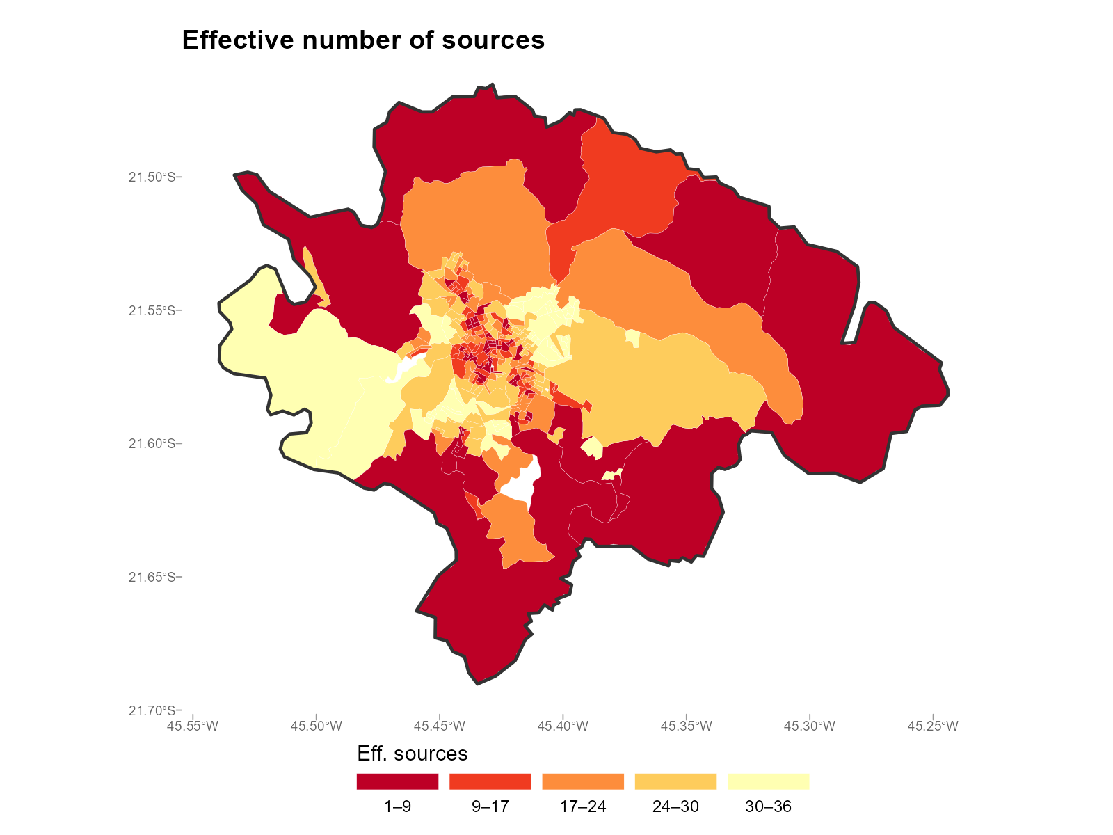

Large city comparison:

plot_weights(result_bh, type = "entropy")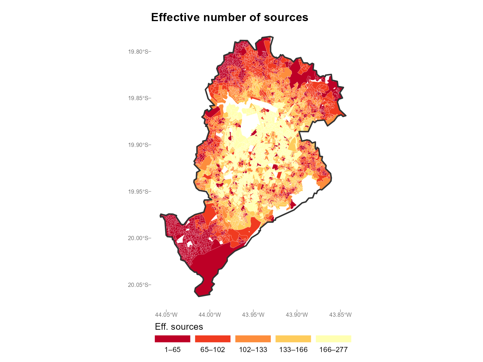

Interactive version (click tracts to see weight summary stats):

plot_weights(result_bh, type = "entropy", interactive = TRUE)

Dominant station map: `plot_weights(type = "dominant")`

plot_weights(result_vga, type = "dominant")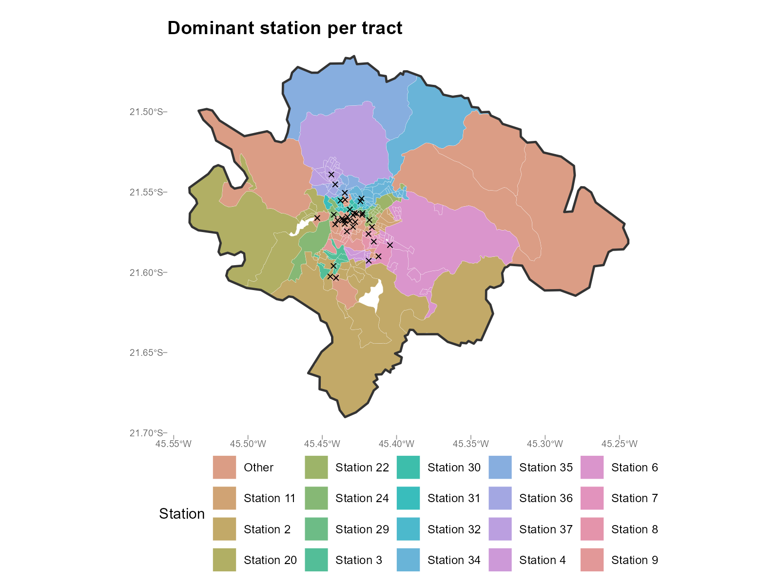

plot_weights(result_nit, type = "dominant")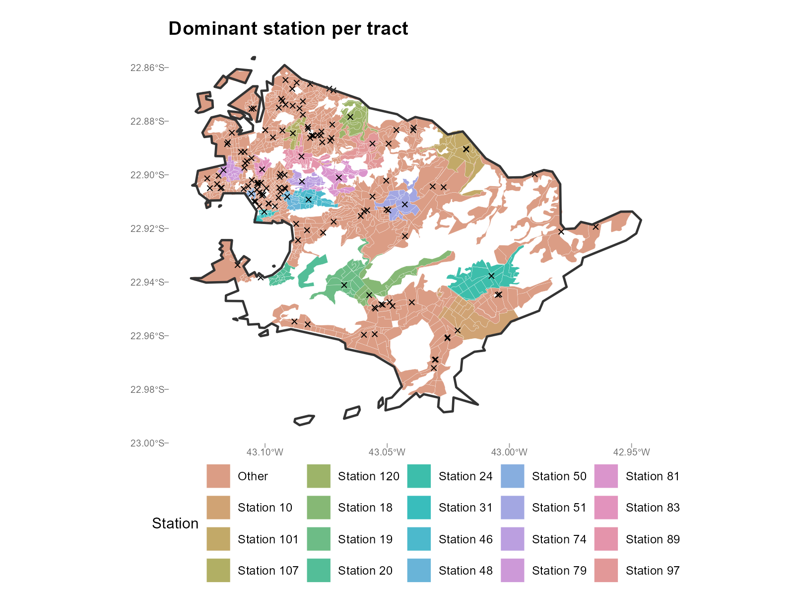

Catchment mode: `plot_weights(type = "catchment")`

Auto-selects the tract with highest effective number of sources:

plot_weights(result_vga, type = "catchment")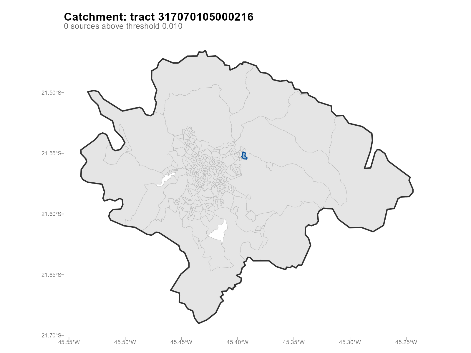

Filtered view with top_k and threshold:

plot_weights(result_vga, type = "catchment", tract = 1,
             top_k = 3, threshold = 0.05)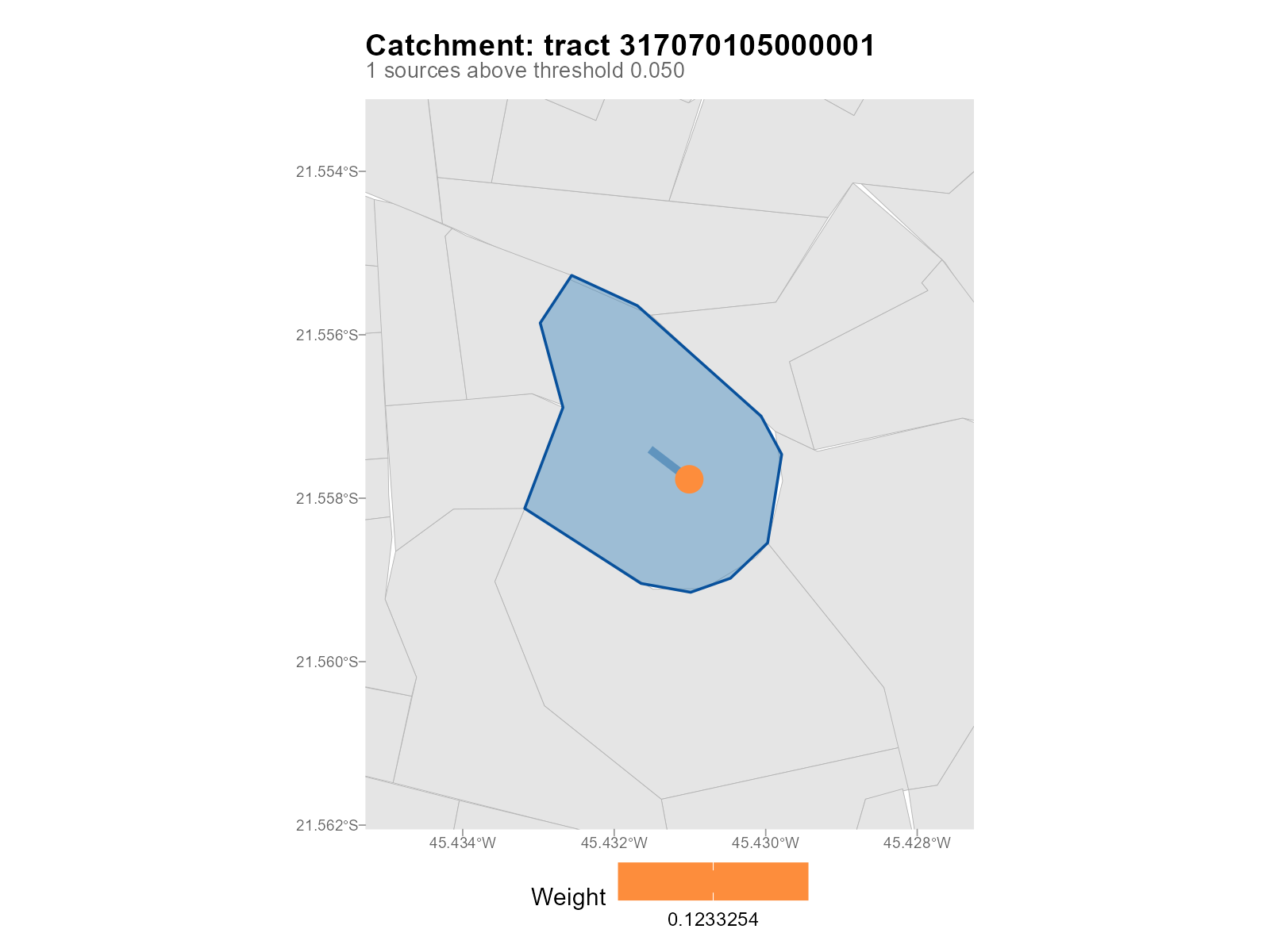

Connections: `plot_connections()`

Overview — one spoke per tract to its dominant station:

plot_connections(result_vga)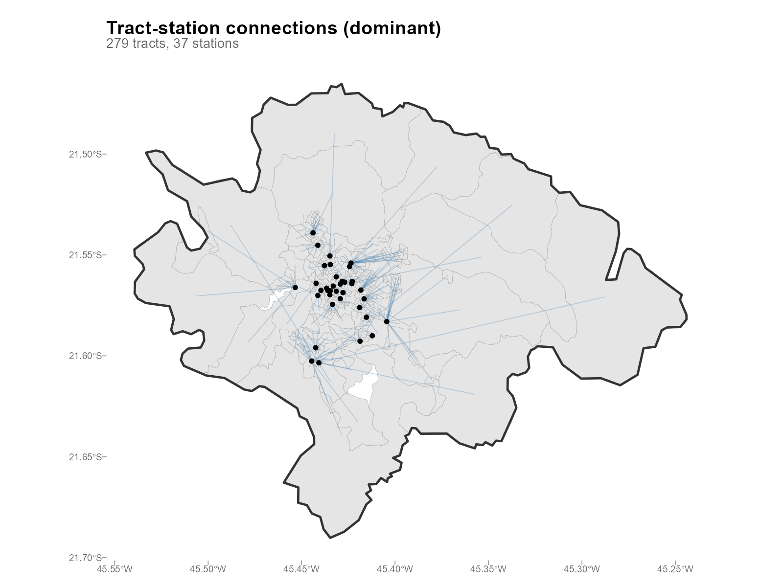

Large city:

plot_connections(result_bh)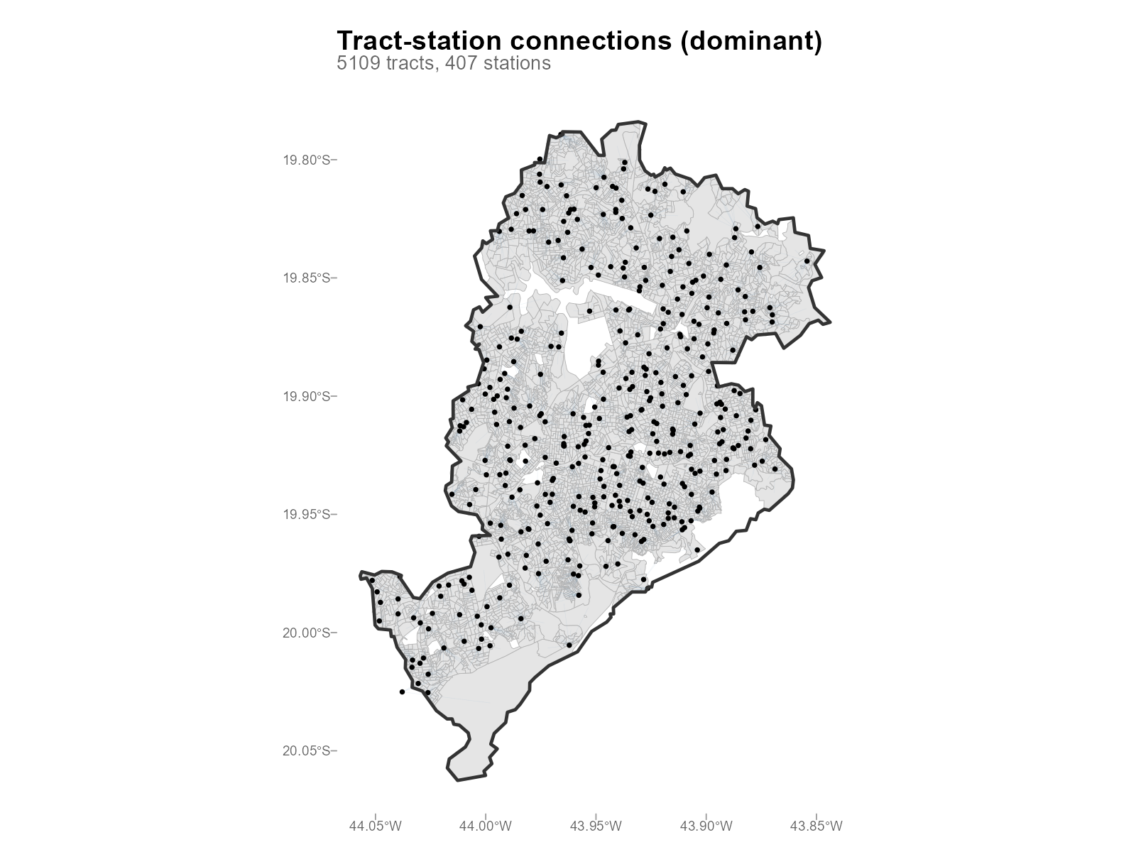

Interactive version for BH (click tracts and stations for detailed weight tables):

Detail for a specific tract:

plot_connections(result_vga, tract = 1)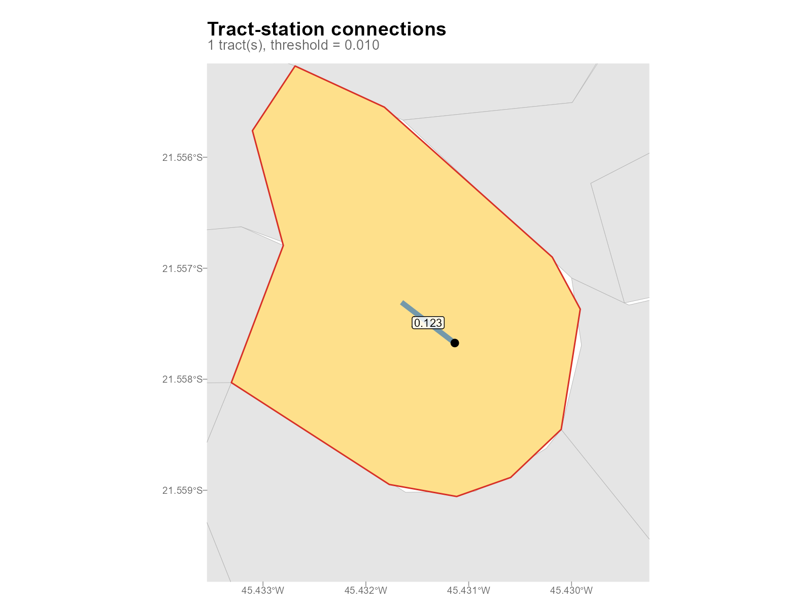

Interactive exploration

All weight diagnostics support interactive = TRUE, which produces leaflet/mapview maps with rich click popups. This is the recommended way to explore the weight structure for individual tracts and stations.

Interactive connections — click any tract to see its top-5 connected stations (with weights, travel times, and cumulative weight). Click any station to see which tracts it serves:

plot_connections(result_vga, interactive = TRUE)

Interactive dominant station map — click any tract to see weight summary statistics (effective sources, HHI, dominant weight):

plot_weights(result_vga, type = "dominant", interactive = TRUE)

Interpretation

Effective number of sources: This is the exponential of Shannon entropy on the row-normalized weights. A value of 1 means the tract depends on a single station; a value of 10 means the weights are equivalent to 10 equal-weight stations. High values (e.g., > 50) can indicate that distant stations are receiving non-negligible weight. The default max_trip_duration = 180 (3 hours walking) and fill_missing = NA policy (see Section 6) address this by assigning exactly zero weight to unreachable and distant pairs.
Low entropy tracts (effective N close to 1): The interpolation for this tract depends almost entirely on a single station. If that station’s data is atypical, the interpolated values may be unreliable.
Dominant station map: Produces a Voronoi-like partition. If catchment areas don’t match geographic intuition, check the travel time matrix.
Connections: The spoke pattern should make geographic sense — tracts should connect to nearby stations. Long-distance connections suggest routing issues.

6. Travel Time Data Quality: `plot_travel_times()`

Intuition

The travel time matrix is the input that drives everything: $\alpha$ optimization, weight computation, and ultimately the spatial allocation of voters. Poor travel time data (unreachable pairs, disconnected road networks) directly degrades interpolation quality.

Applied examples

Histogram — distribution of all $n \times m$ travel times:

plot_travel_times(result_vga, type = "histogram")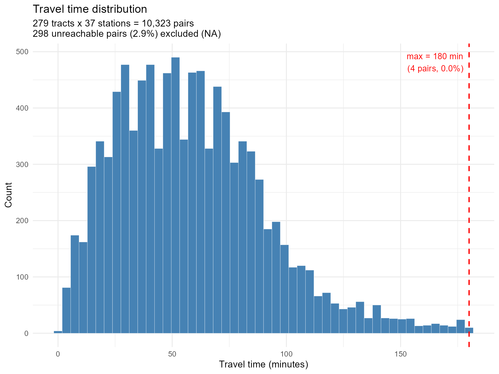

Large city:

plot_travel_times(result_bh, type = "histogram")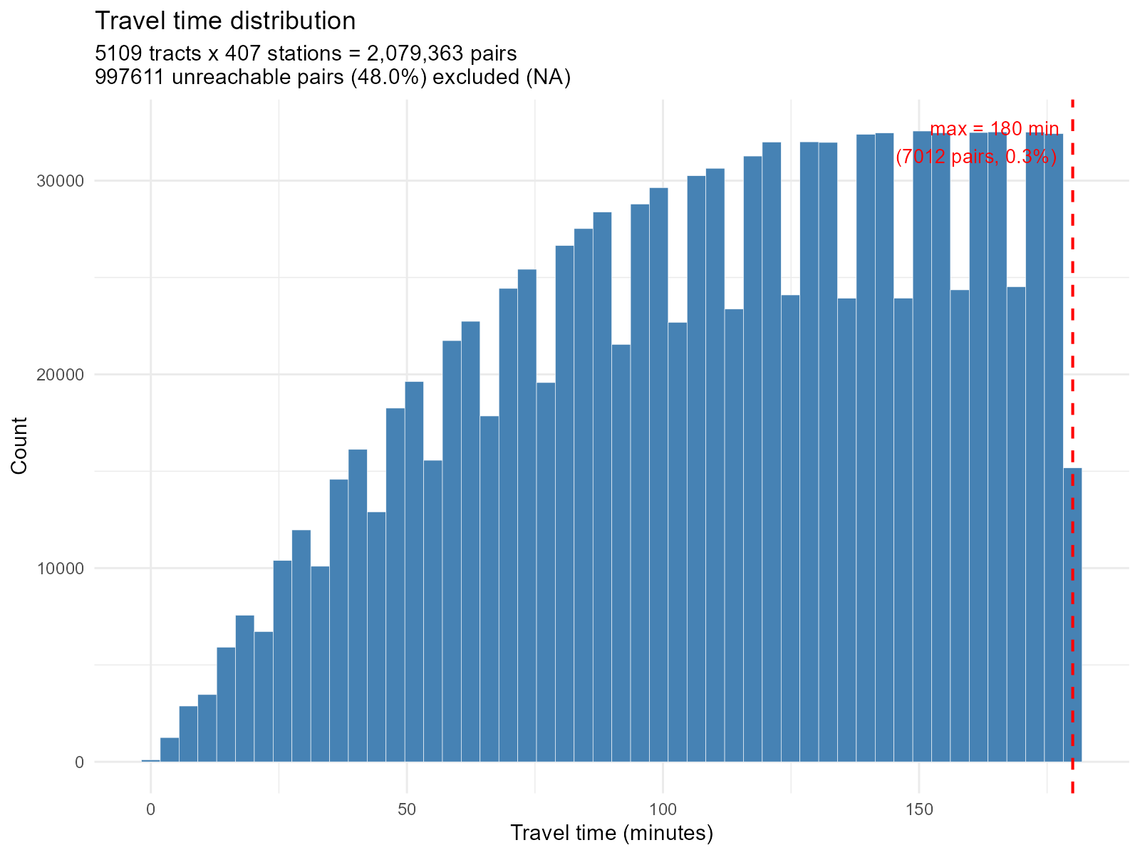

Heatmap — rows = tracts (ordered by latitude), columns = stations. Block-diagonal structure reveals spatial locality:

plot_travel_times(result_vga, type = "heatmap")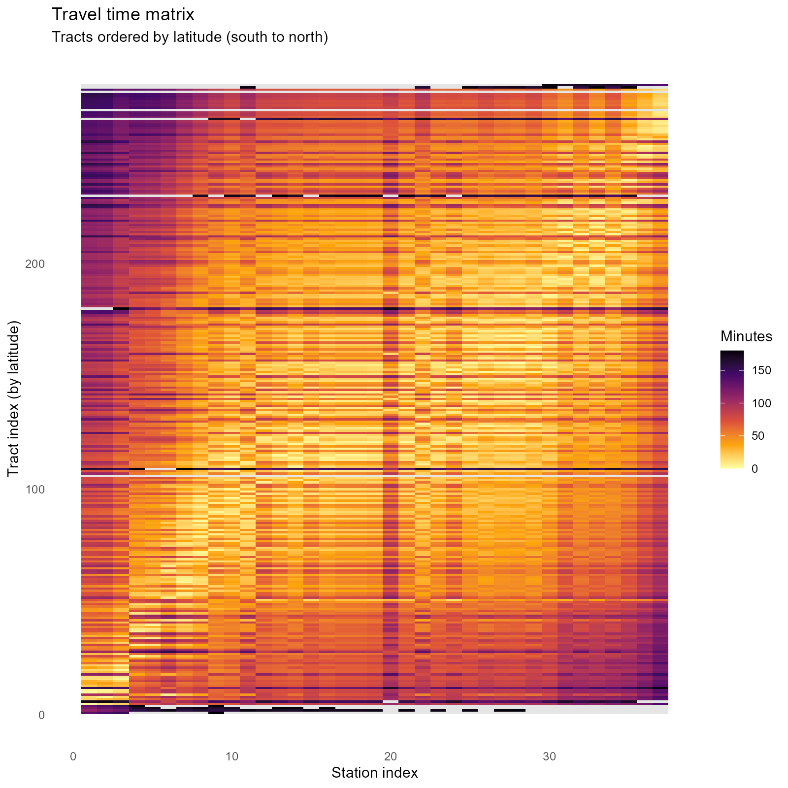

Map — station points colored by travel time for a specific tract:

plot_travel_times(result_vga, type = "map", tract = 1)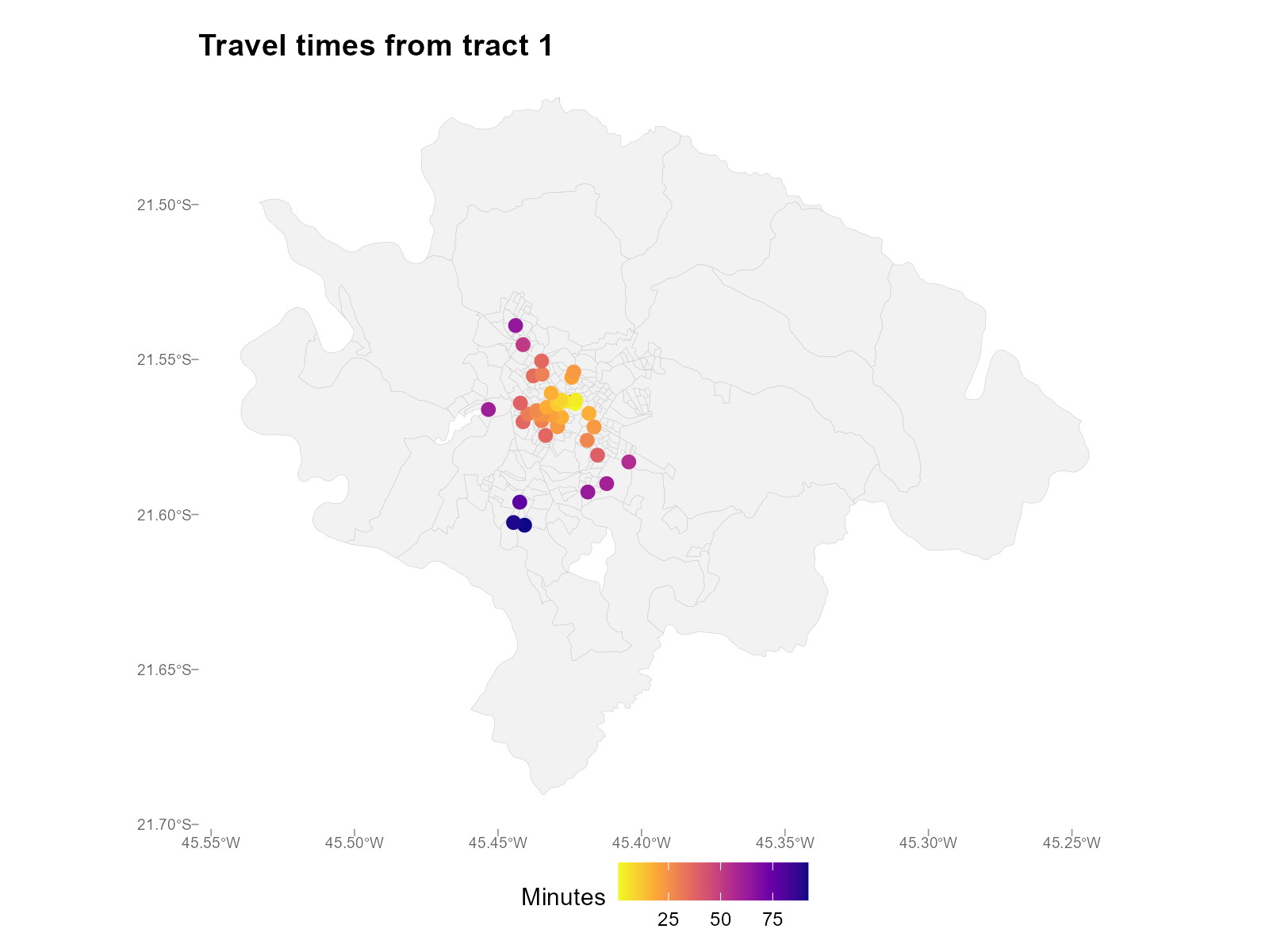

Unreachable pairs and the `fill_missing` parameter

When the routing engine cannot find a path between a tract and a station within max_trip_duration minutes, the travel time is NA. By default, routing_control(fill_missing = NULL) resolves to NA, which means these unreachable pairs remain as NA in the travel time matrix and receive exactly zero weight — they are completely excluded from both the optimization and the interpolation.

The default max_trip_duration = 180 (3 hours walking) intentionally cuts distant links. Any tract–station pair beyond this threshold is treated as unreachable. This prevents distant stations from creating a uniform background weight that inflates the effective number of sources.

If a tract has no reachable stations at all (entire row is NA), it is excluded from optimization and receives NA interpolated values.

To assign a finite fill value instead (e.g., to ensure every pair has a travel time):

routing_control(fill_missing = 300)  # fill unreachable with 300 min

Interpretation

NA pairs in histogram: The subtitle reports how many pairs are unreachable (NA). A large number suggests poor OSM network coverage or a restrictive max_trip_duration.
Grey cells in heatmap: Represent NA (unreachable) pairs. These receive zero weight.
Bimodal distribution: May indicate disconnected graph components (e.g., separated by a river without bridge in the OSM network).
Block-diagonal heatmap: Expected — nearby tracts have similar travel times to the same stations. Absence of block structure suggests the travel times lack spatial coherence.

7. Spatial Autocorrelation: `plot_residual_autocorrelation()` + `plot_moran()`

Intuition

Residual autocorrelation: If residuals are spatially clustered (nearby tracts have similar residuals), the model is missing spatial structure — a misspecification signal.

Moran’s I on interpolated variables: If the interpolated vote shares show expected spatial concentration (e.g., PT strongholds in low-income areas), the method is preserving realistic political geography.

Formal definition

Global Moran’s I: $I = \frac{n}{\sum_{i,j} w_{ij}} \cdot \frac{\sum_{i,j} w_{ij}(x_i - \bar{x})(x_j - \bar{x})}{\sum_i (x_i - \bar{x})^2}$

where $w_{ij}$ are spatial weights (queen contiguity). Range: $[-1, +1]$ . Positive = clustering, $\approx 0$ = random, negative = dispersion.

LISA (Local Moran’s I): $I_i = \frac{(x_i - \bar{x})}{s^2} \sum_j w_{ij}(x_j - \bar{x})$ . Classification: HH (high-high cluster), LL (low-low), HL (high surrounded by low), LH (low surrounded by high).

Applied examples: Residual autocorrelation

plot_residual_autocorrelation(result_vga)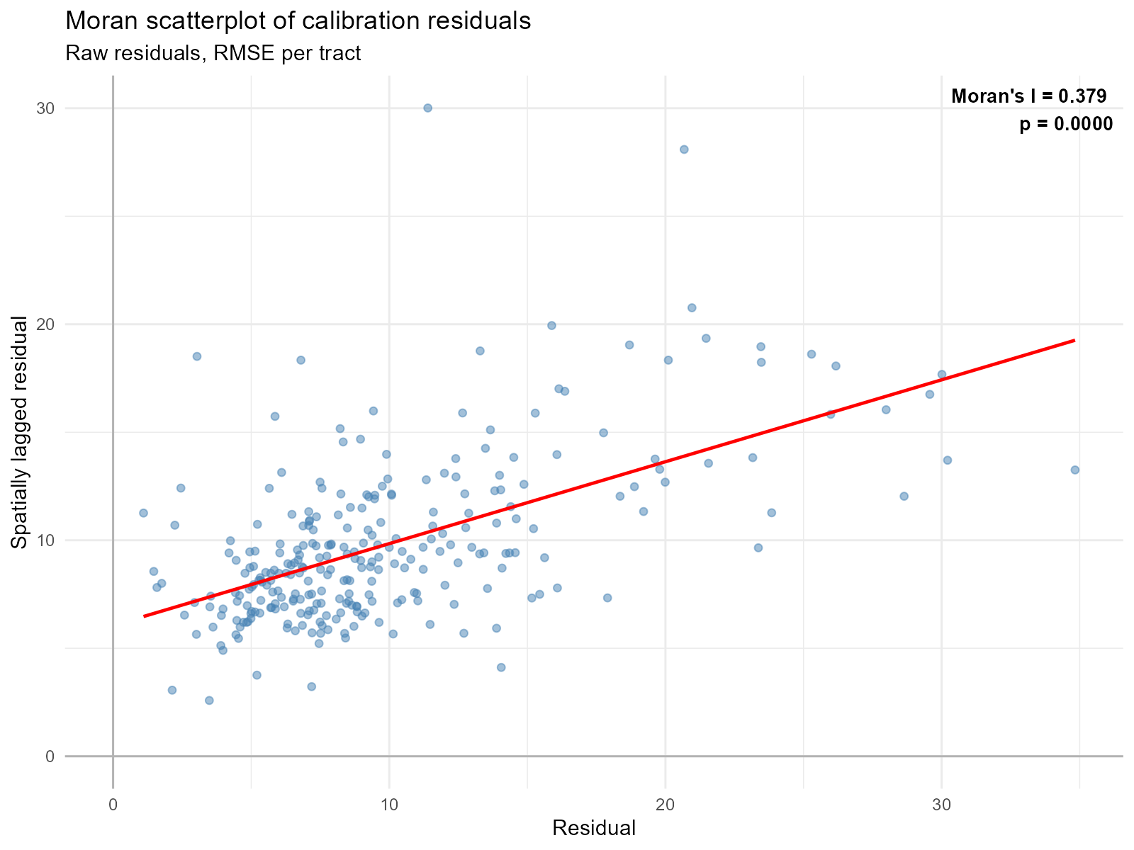

Pearson residuals:

plot_residual_autocorrelation(result_vga, residual_type = "pearson")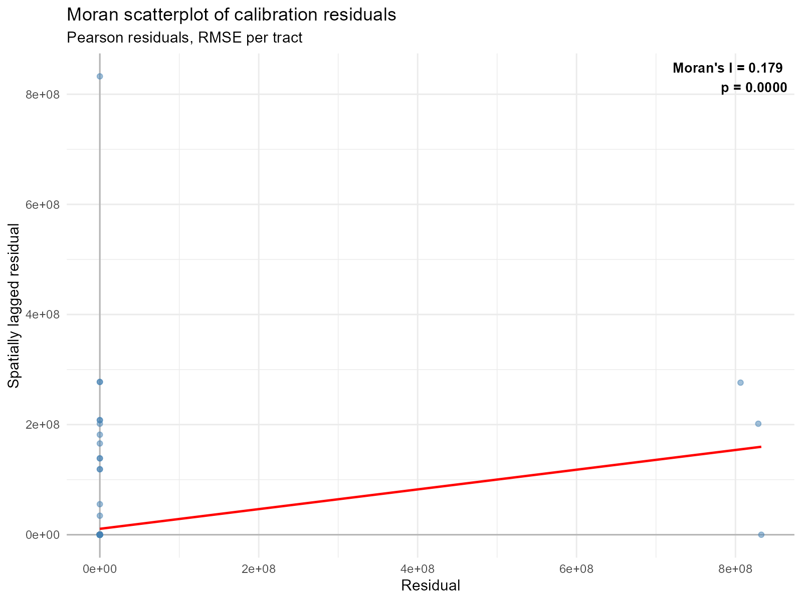

Applied examples: LISA cluster maps

plot_moran(result_vga, variable = "Lula", type = "lisa")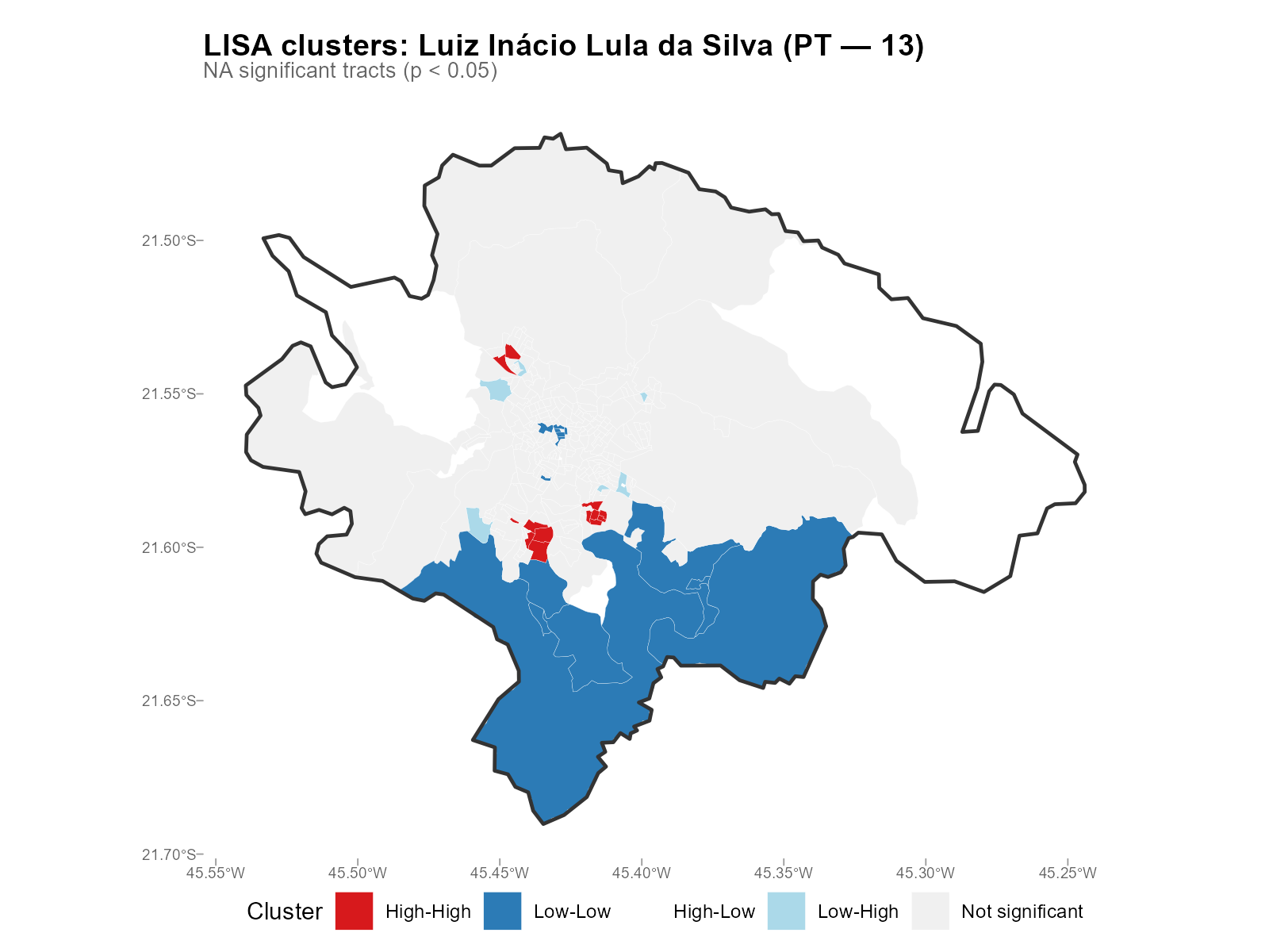

Moran scatterplot:

plot_moran(result_vga, variable = "Lula", type = "moran")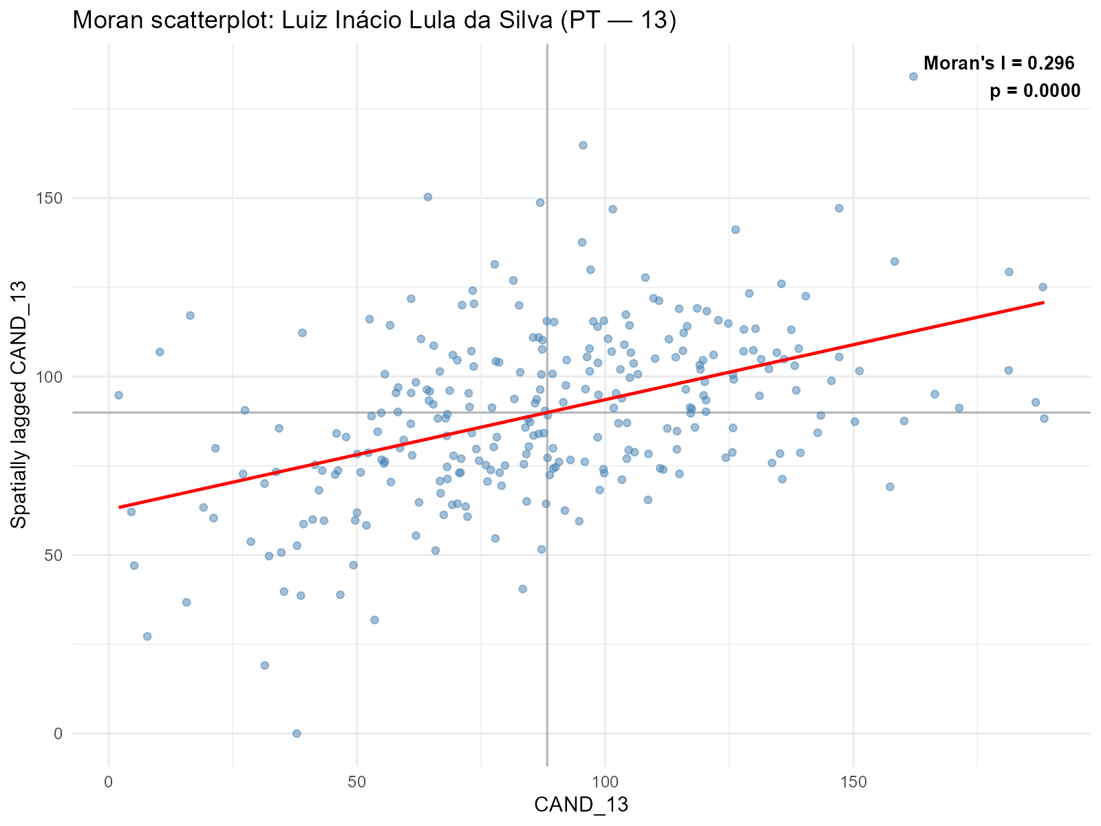

Large city:

plot_moran(result_bh, variable = "Lula", type = "lisa")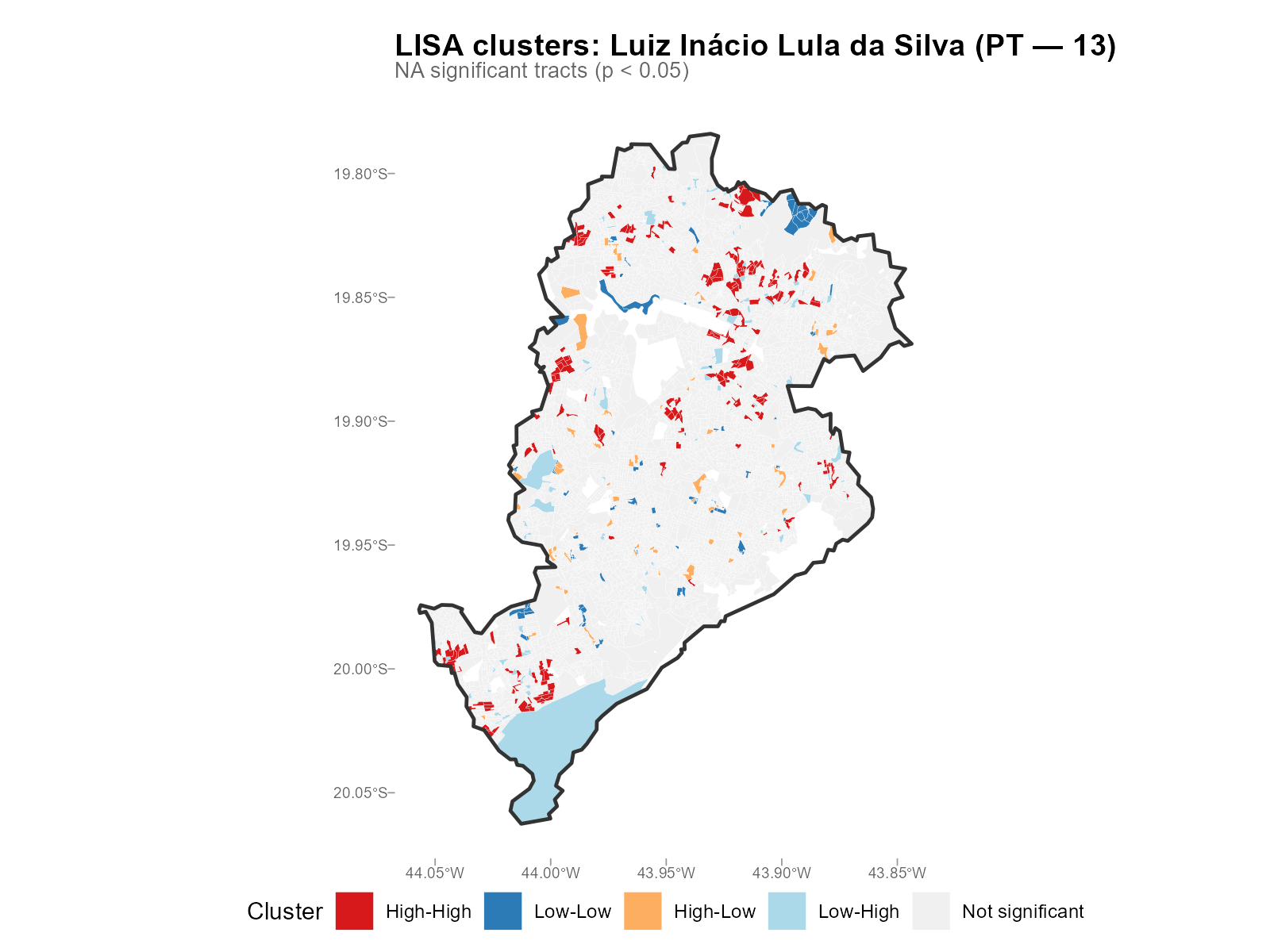

By party:

plot_moran(result_nit, variable = "PT", type = "lisa")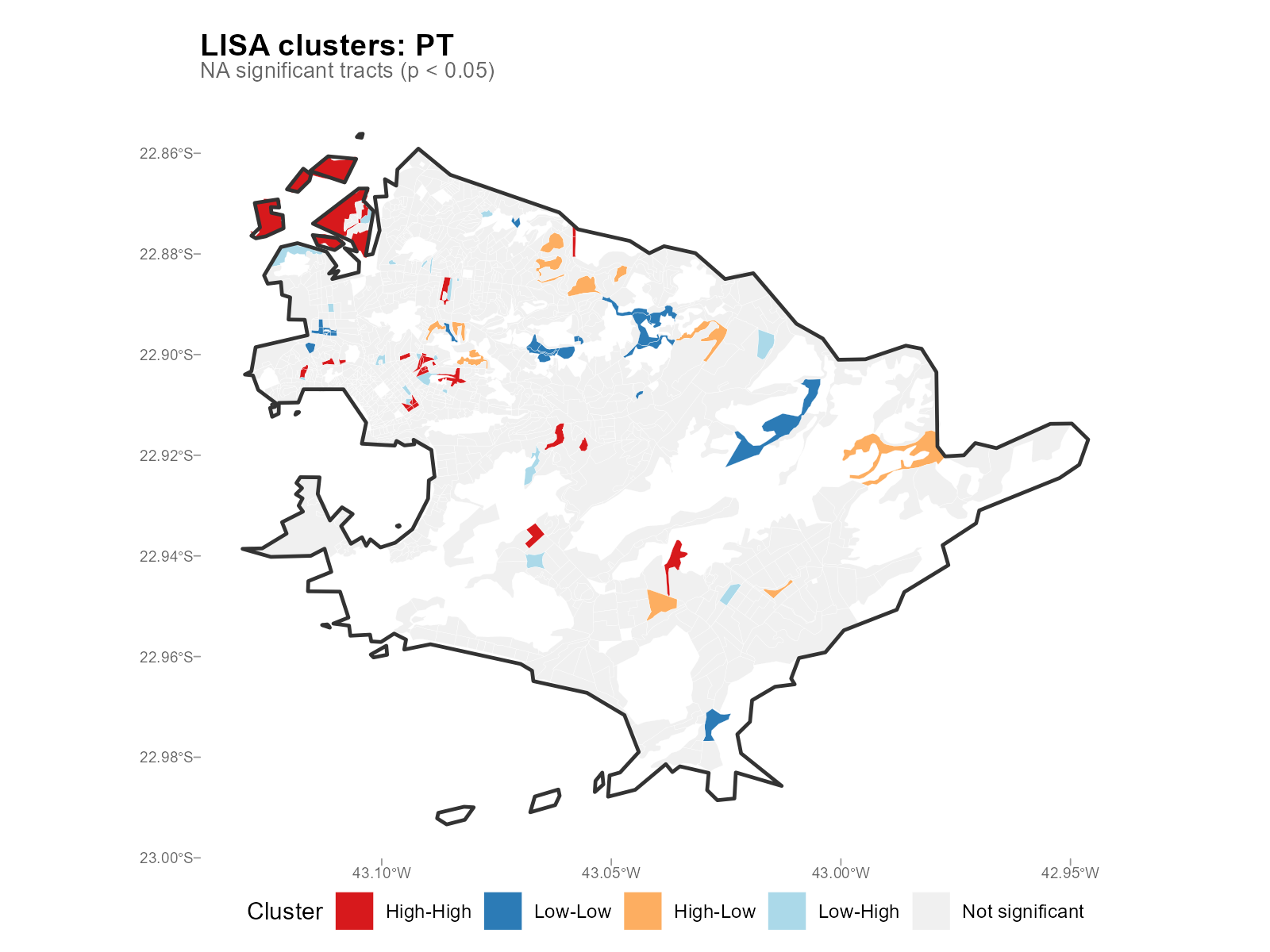

Interpretation

Significant Moran’s I on residuals (p < 0.05): The model has spatially structured error. Consider whether the travel time data has systematic problems in certain areas.
HH clusters of Lula votes: Expected in low-income neighborhoods (PT strongholds). Their presence validates that the interpolation preserves known political geography.
HL/LH clusters: Spatial outliers — tracts with high vote share surrounded by low (or vice versa). May indicate local effects or data irregularities.

8. Ecological Validation

8a. Implied Turnout Rates: `plot_turnout_rates()`

Intuition

For each tract and demographic bracket, the implied turnout rate is:

$\text{rate}_{i,b} = \frac{\text{fitted voters}_{i,b}}{\text{census population}_{i,b}}$

In Brazil, voting is compulsory for ages 18–69, so expected turnout is ~75–85%. For 16–17 and 70+, voting is optional and rates should be lower. Rates exceeding 100% indicate tracts where the model allocates more voters than residents — signaling boundary effects or registration mismatches.

Applied examples

Bracket boxplot:

plot_turnout_rates(result_vga, type = "bracket")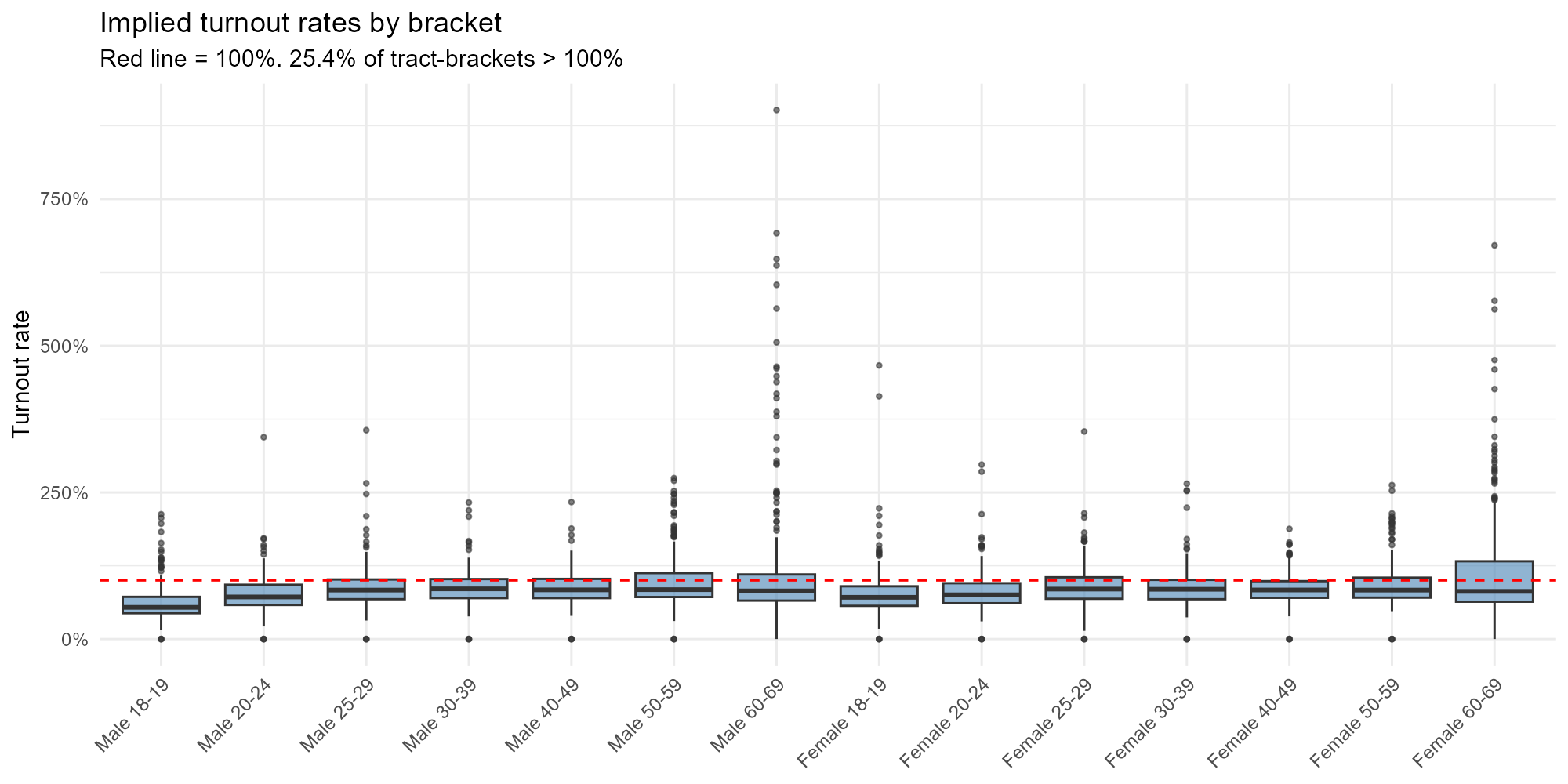

plot_turnout_rates(result_nit, type = "bracket")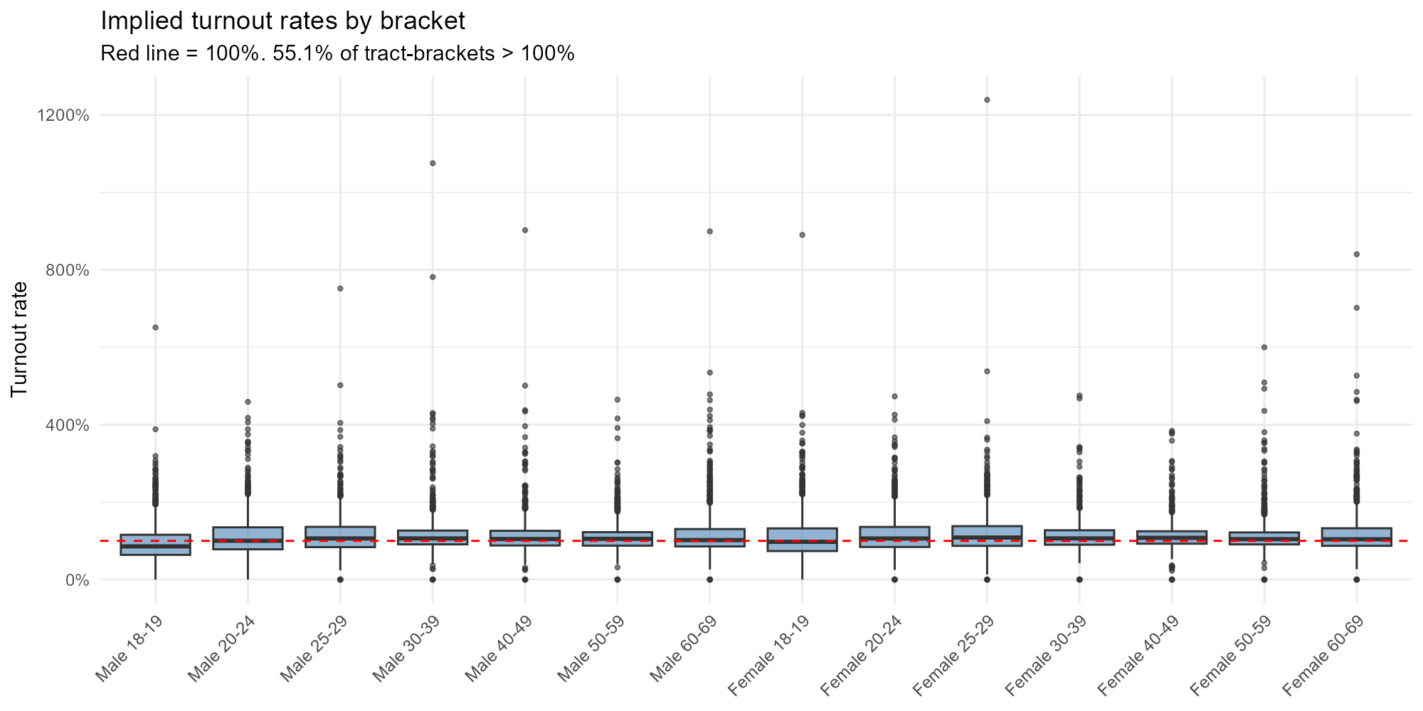

Spatial pattern:

plot_turnout_rates(result_bh, type = "map")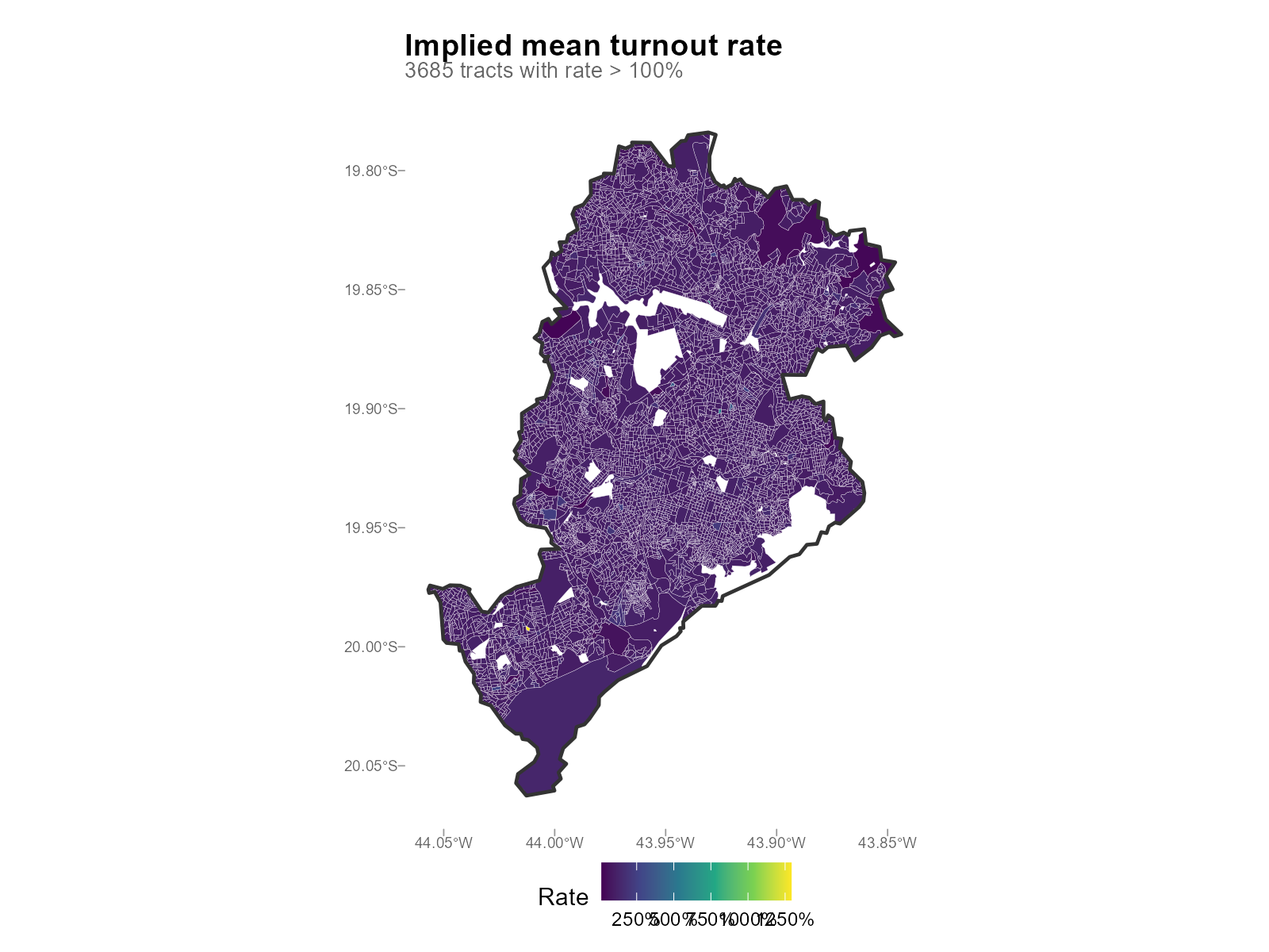

Faceted histogram:

plot_turnout_rates(result_vga, type = "histogram")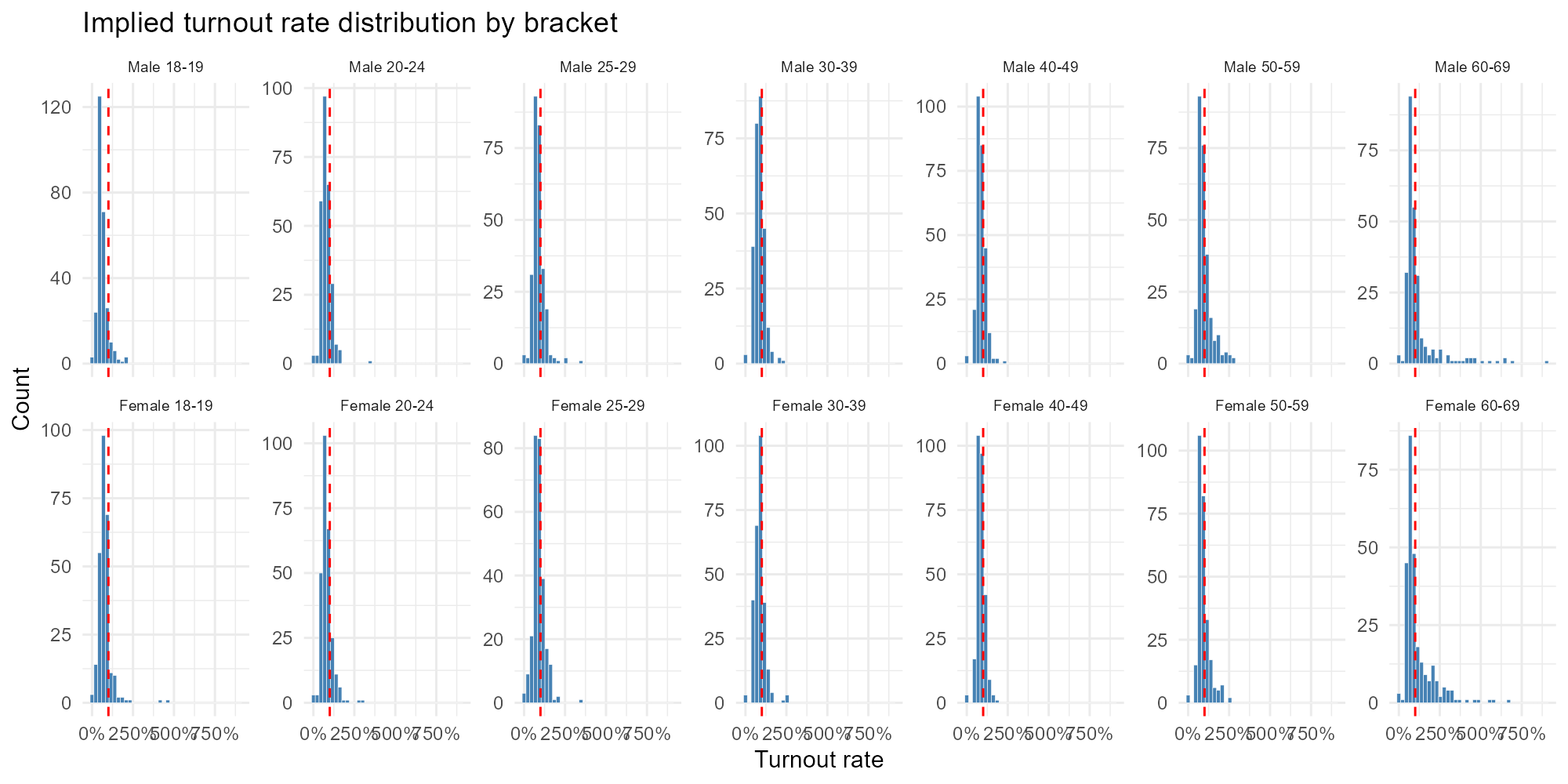

Interpretation

Compulsory brackets clustering around 80%: Expected for ages 18–69.
Optional brackets lower: 16–17 and 70+ should show lower turnout.
Rates > 100%: Voters registered in one municipality who may actually reside in another (commuters, students). These boundary effects are a known limitation of the model.

8b. Income-Vote Correlation: `plot_income()`

Intuition

The negative correlation between PT vote share and income is one of the best-documented patterns in Brazilian political science (the “PT-income gradient”). If the interpolation preserves this gradient, it builds confidence that the spatial allocation of votes is realistic. If it destroys it, something is wrong.

Income data comes from censobr (Census Bureau microdata), which provides mean household head income by tract. No deflation is applied — within a single census year, the correlation is scale-invariant.

Applied examples

Lula (PT) vs income — expect negative correlation:

plot_income(result_vga, variable = "Lula", type = "scatter")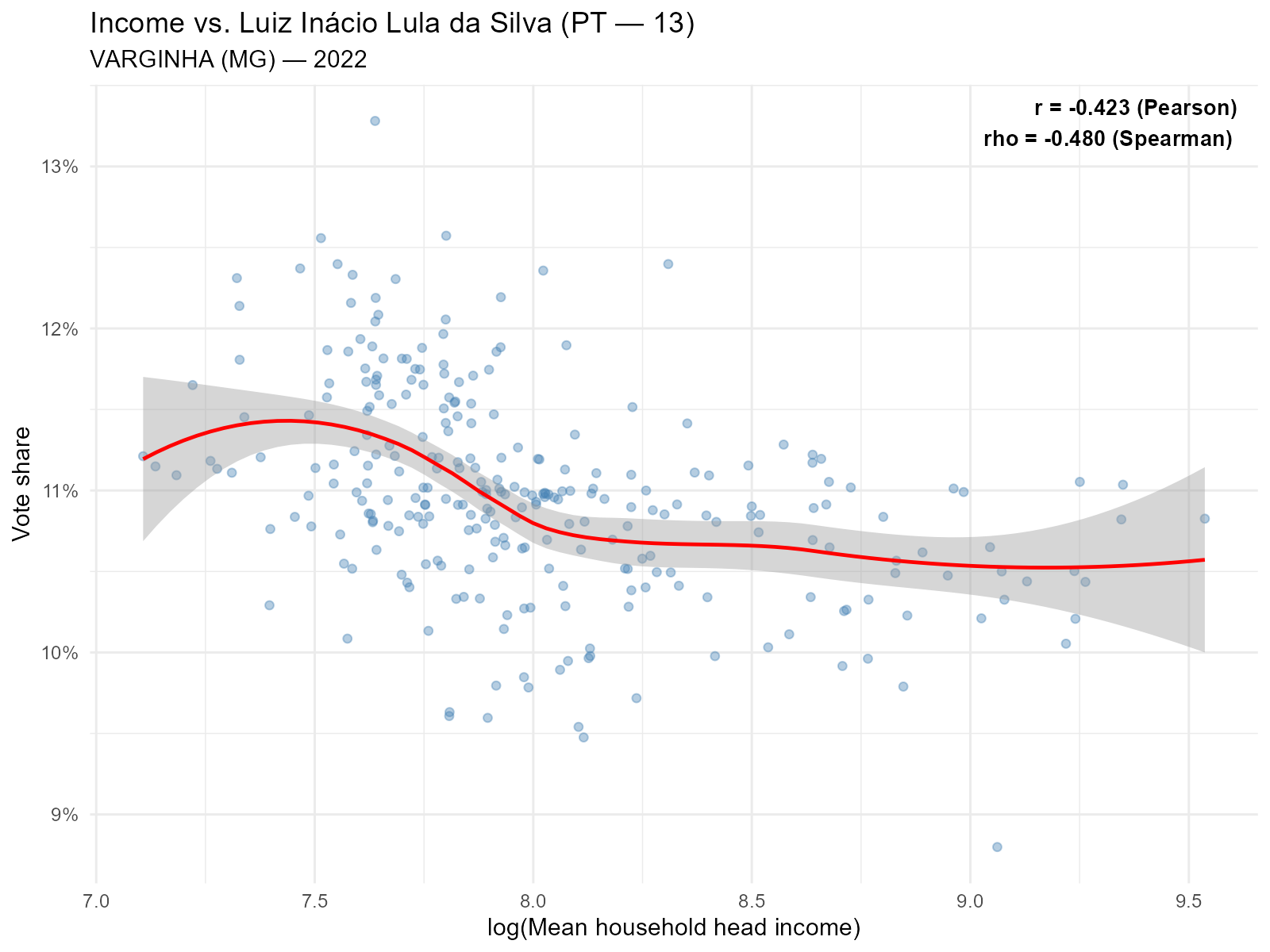

Bolsonaro (PL) vs income — expect positive correlation:

plot_income(result_vga, variable = 22, type = "scatter")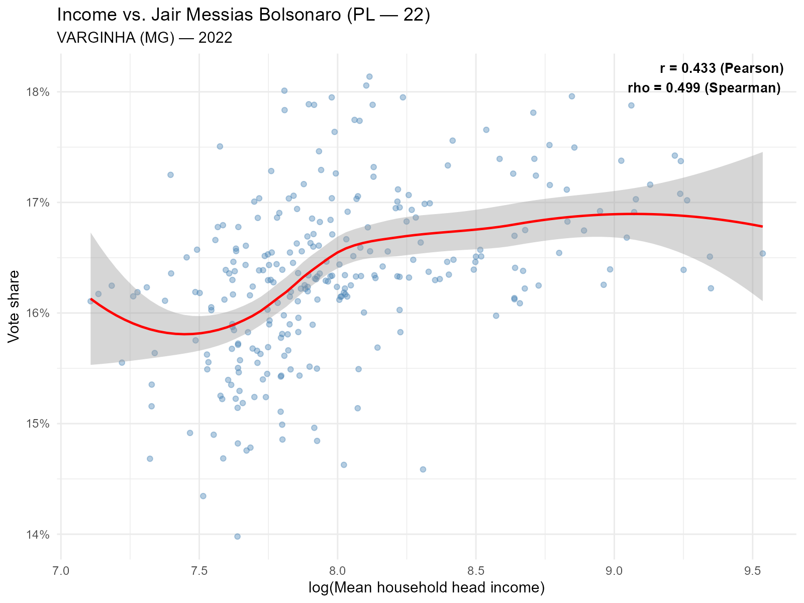

Larger city:

plot_income(result_bh, variable = "Lula", type = "scatter")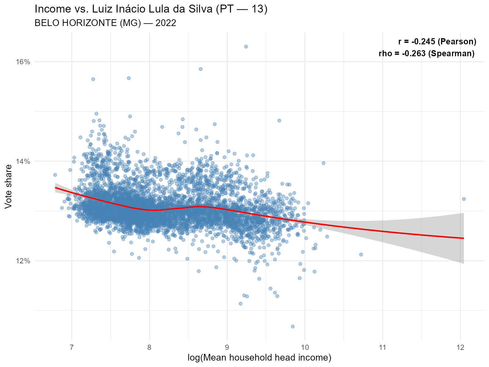

Side-by-side maps:

plot_income(result_nit, variable = "Lula", type = "map")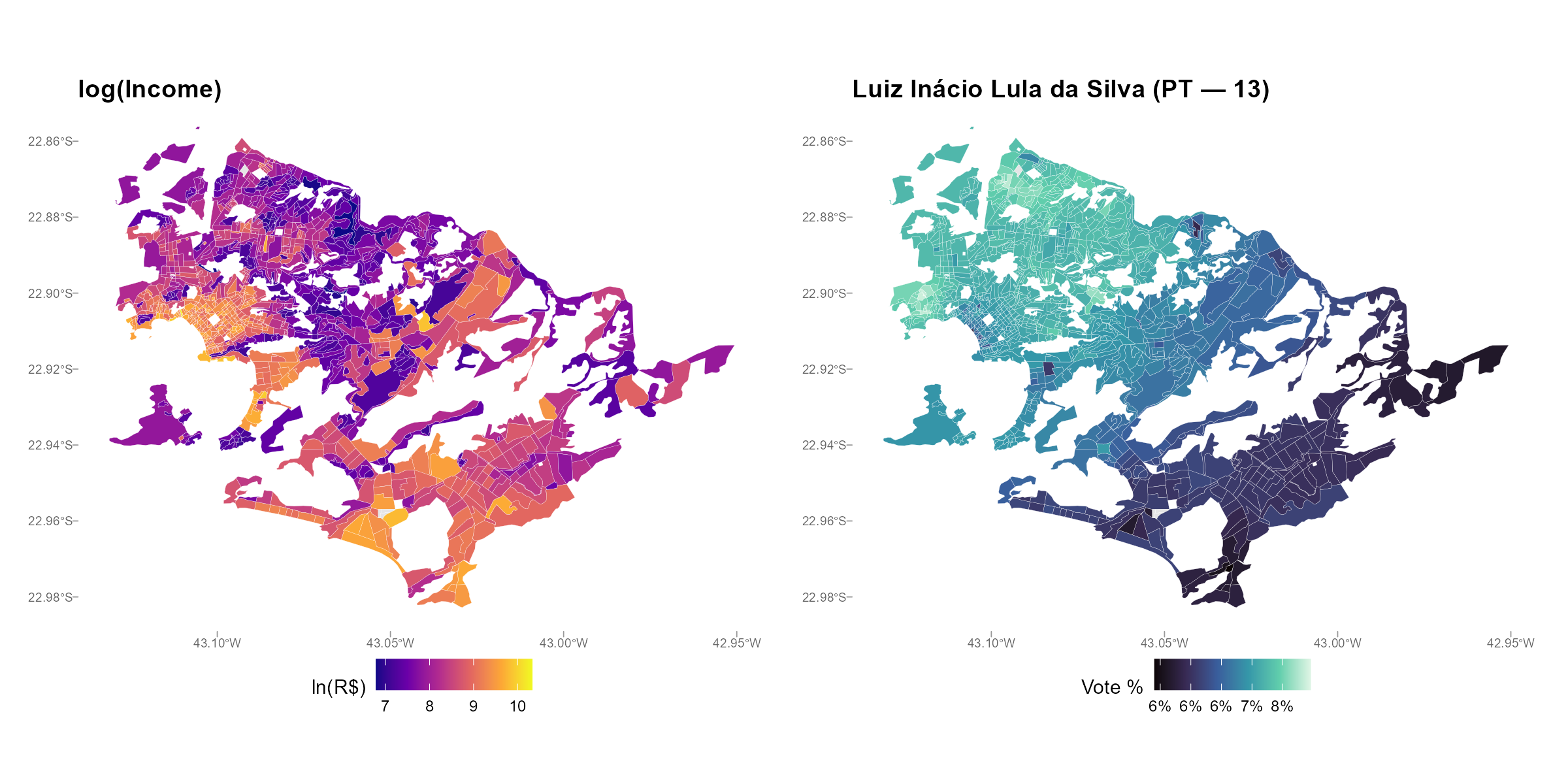

8c. Cross-Round Consistency: `plot_ecological()`

Intuition

Political geography is sticky. Neighborhoods that vote strongly for a candidate in round 1 should vote even more strongly in round 2 (where only 2 candidates remain). A high correlation between turno 1 and turno 2 tract-level vote shares validates that the interpolation preserves spatial patterns.

Applied examples

plot_ecological(result_vga, result_vga2,
                variable = "Lula", type = "scatter")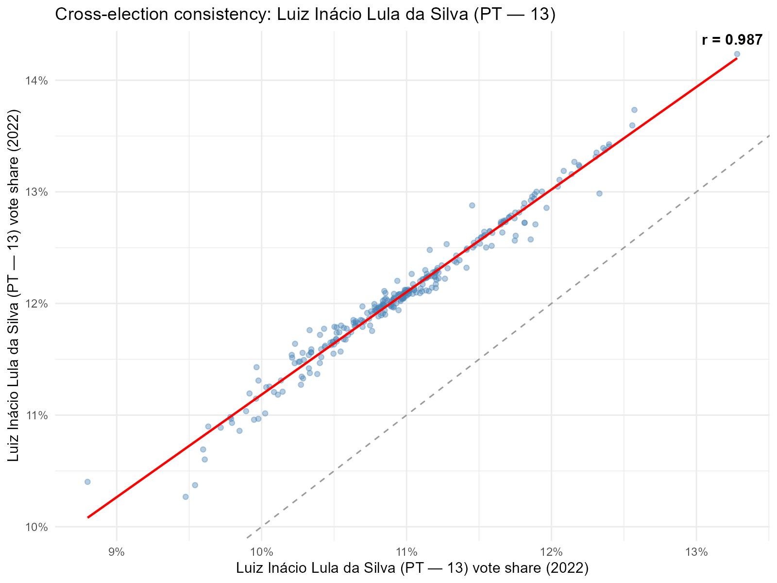

Side-by-side maps:

plot_ecological(result_vga, result_vga2,
                variable = "Lula", type = "map")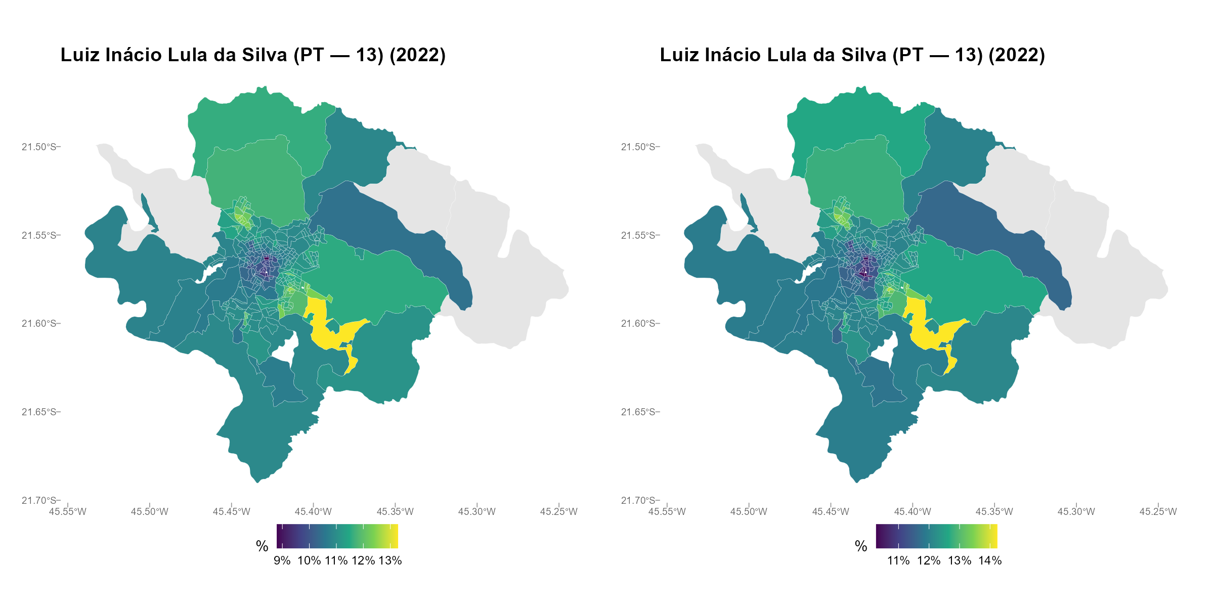

Interpretation

Strong positive correlation between rounds: The spatial patterns are consistent, as expected. The method is recovering stable partisan geography.
Weak or no correlation: The interpolation may be injecting noise rather than recovering signal. Investigate whether the travel time data or optimization is causing problems.

9. Quick Reference

Function	Question it answers	Key arguments	When to worry
`diagnostics()`	Is anything obviously wrong?	`verbose`	Any FAIL or multiple WARNs
`plot_convergence()`	Did the optimizer converge?	`which`, `log_y`	Oscillating loss, non-shrinking gradient
`plot_alpha()`	How does distance decay vary?	`type`, `summary_fn`, `brackets`	Many tracts with $\alpha > 15$
`plot_residuals()`	How well are demographics reproduced?	`type`, `residual_type`, `summary_fn`	Large systematic bias, Pearson > 3
`residual_summary()`	Which brackets/tracts fit worst?	`type`	One bracket much worse than others
`weight_summary()`	How concentrated are the weights?	—	Many tracts with effective N = 1
`plot_weights()`	Where are catchment areas?	`type`, `tract`, `top_k`	Catchments that defy geography
`plot_connections()`	Which stations serve which tracts?	`tract`, `top_k`, `threshold`	Long-distance connections
`plot_travel_times()`	Is the travel time matrix clean?	`type`, `tract`	Large spike at max value
`plot_residual_autocorrelation()`	Are residuals spatially clustered?	`residual_type`, `summary_fn`	Significant Moran’s I (p < 0.05)
`plot_moran()`	Is vote geography realistic?	`variable`, `type`	No spatial clustering
`plot_turnout_rates()`	Are implied turnout rates plausible?	`type`	Many tracts > 100%
`plot_income()`	Does the PT-income gradient hold?	`variable`, `type`	Wrong sign on correlation
`plot_ecological()`	Are spatial patterns consistent?	`variable`, `type`	Weak cross-round correlation

Setup

1. Automated Health Check: diagnostics()

Intuition

Formal definition

Applied example

Interpretation

2. Optimization Convergence: plot_convergence()

Intuition

Formal definition

Applied examples

Interpretation

3. Alpha Decay Parameters: plot_alpha()

Intuition

Formal definition

Applied examples: Map mode

Applied examples: Histogram mode

Applied examples: Bracket boxplot

Interpretation

4. Calibration Residuals: plot_residuals() + residual_summary()

Intuition

Formal definition

Applied examples: Map mode

Applied examples: Histogram mode

Applied examples: Bracket boxplot

Applied examples: Scatter (fitted vs observed)

Tabular summary: residual_summary()

Interpretation

5. Weight Structure

Intuition

Formal definition

Tabular summary: weight_summary()

Entropy map: plot_weights(type = "entropy")

Dominant station map: plot_weights(type = "dominant")

Catchment mode: plot_weights(type = "catchment")

Connections: plot_connections()

Interactive exploration

Interpretation

6. Travel Time Data Quality: plot_travel_times()

Intuition

Applied examples

Unreachable pairs and the fill_missing parameter

Interpretation

7. Spatial Autocorrelation: plot_residual_autocorrelation() + plot_moran()

Intuition

Formal definition

Applied examples: Residual autocorrelation

Applied examples: LISA cluster maps

Interpretation

8. Ecological Validation

8a. Implied Turnout Rates: plot_turnout_rates()

Intuition

Applied examples

Interpretation

8b. Income-Vote Correlation: plot_income()

Intuition

Applied examples

8c. Cross-Round Consistency: plot_ecological()

Intuition

Applied examples

Interpretation

9. Quick Reference

1. Automated Health Check: `diagnostics()`

2. Optimization Convergence: `plot_convergence()`

3. Alpha Decay Parameters: `plot_alpha()`

4. Calibration Residuals: `plot_residuals()` + `residual_summary()`

Tabular summary: `residual_summary()`

Tabular summary: `weight_summary()`

Entropy map: `plot_weights(type = "entropy")`

Dominant station map: `plot_weights(type = "dominant")`

Catchment mode: `plot_weights(type = "catchment")`

Connections: `plot_connections()`

6. Travel Time Data Quality: `plot_travel_times()`

Unreachable pairs and the `fill_missing` parameter

7. Spatial Autocorrelation: `plot_residual_autocorrelation()` + `plot_moran()`

8a. Implied Turnout Rates: `plot_turnout_rates()`

8b. Income-Vote Correlation: `plot_income()`

8c. Cross-Round Consistency: `plot_ecological()`